Modelling the Otto and Diesel Cycles in Python

Otto Cycle

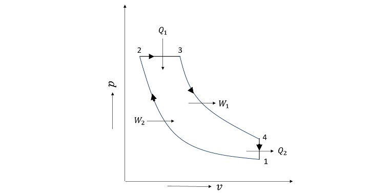
An air standard cycle called the Otto Cycle is employed in spark ignition (SI) engines. It comprises of two reversible adiabatic processes and two isochoric processes (constant volume), totaling four processes. When the work interactions take place in reversible adiabatic processes, the heat addition (2-3) and rejection (4-1) occur isochorically (3-4 and 1-2). The Otto cycle's schematic is shown in Figure given below.

To model the cycle in Python, the input variables considered are maximum pressure $\mathrm{(P_{max})}$, minimum pressure $\mathrm{(P_{min})}$, maximum volume $\mathrm{(V_{max})}$, compression ratio (r), and adiabatic exponent $\mathrm{(\gamma)}$. Table 2 explains the thermodynamic computations of different processes involved in the Otto cycle −

Process 1-2

$$\mathrm{p_{1} \: = \: p_{min}}$$

$$\mathrm{v_{1} \: = \: v_{max}}$$

Using compression ratio (𝑟), first the volume at point 2 will be evaluated based on the volume at point 1 as −

$$\mathrm{v_{2} \: = \: \frac{v_{1}}{r}}$$

Then the adiabatic constant along the process 1-2 is evaluated as −

$$\mathrm{c_{1} \: = \: p_{1} \: \times \: v_{1}^{\gamma}}$$

Once $\mathrm{c_{1}}$ is known, the pressure variation along the line 1-2 is evaluated as −

$$\mathrm{p \: = \: \frac{c_{1}}{v^{\gamma}}}$$

Process 2-3

$$\mathrm{p_{3} \: = \: p_{max}}$$

As the process is isochoric, so the volume remains the same thus −

$$\mathrm{v_{3} \: = \: v_{2}}$$

Therefore, the pressure at point 2 can be evaluated as −

$$\mathrm{p_{2} \: = \: \frac{c_{1}}{v^{\gamma}_{2}}}$$

Process 3-4

Let $\mathrm{c_{2}}$ be the constant along line 3-4. As pressure and temperature at point 3 are known, so the constant along the reversible adiabatic line can be evaluated as −

$$\mathrm{c_{2} \: = \: p_{3} \: \times \: v_{3}^{\gamma}}$$

And as $\mathrm{v_{4} \: = \: v_{1}}$, so the pressure along 3-4 can be evaluated as −

$$\mathrm{p \: = \: \frac{c_{2}}{v^{\gamma}}}$$

Process 4-1

$\mathrm{c_{2}}$ and $\mathrm{c_{4}}$ are already known so $\mathrm{p_{4}}$ can be evaluated as

$$\mathrm{p_{4} \: = \: \frac{c_{4}}{v^{\gamma}_{4}}}$$

Python Program for the Otto Cycle

The Python function for the Otto cycle is as follows −

from pylab import *
from pandas import *
def otto(p_min,p_max,v_max,r,gma):
font = {'family' : 'Times New Roman','size' : 39}
figure(figsize=(20,15))
rc('font', **font)
'''This function prints Otto cycle
arguments are as follows:
_min: minimum pressure
p_max: Maximum pressure
v_max: Maximum volume
r: compression ratio
gma: Adiabatic exponent
The order of arguments is:
p_min,p_max,v_max,r,gma
'''

#~~~~~~~~~~~~~~~~~~~~~~~~~
# Process 1-2
#~~~~~~~~~~~~~~~~~~~~~~~~~
   p1=p_min
   v1=v_max
   v2=v1/r
   c1=p1*v1**gma
   v=linspace(v2,v1,100)
   p=c1/v**gma
   plot(v,p/1000,'b',linewidth=3)
   
#~~~~~~~~~~~~~~~~~~~~~~~~~
# Process 2-3
#~~~~~~~~~~~~~~~~~~~~~~~~~
   p3=p_max
   v3=v2
   p2=c1/v2**gma
   p=linspace(p2,p3,100)
   v=100*[v3]
   plot(v,p/1000,'r',linewidth=3)
   
#~~~~~~~~~~~~~~~~~~~~~~~~~
# Process 3-4
#~~~~~~~~~~~~~~~~~~~~~~~~~
   c2=p3*v3**gma
   v4=v1
   v=linspace(v3,v4,100)
   p=c2/v**gma
   plot(v,p/1000,'g',linewidth=3)
   
#~~~~~~~~~~~~~~~~~~~~~~~~~
# Process 4-1
#~~~~~~~~~~~~~~~~~~~~~~~~~
   v4=v1
   p4=c2/v4**gma
   p=linspace(p1,p4,100)
   v=100*[v1]
   plot(v,p/1000,'r',linewidth=3)
   title('Otto Cycle',size='xx-large',color='k')
   xlabel('Volume ($m^3$)')
   ylabel('Pressure (kPa)')
   text(v1,p1/1000-30,'1')
   text(v2,p2/1000-200,'2')
   text(v3+0.01,p3/1000-20,'3')
   text(v4,p4/1000+10,'4')
   data={'p':[p1,p2,p3,p4],
      'v':[v1,v2,v3,v4],
      'c':[c1,'' ,c2,'' ],
      'State': [1,2,3,4]}
   df=DataFrame(data)
   savefig('Otto_final.jpg')
   return df.set_index('State')
   oc=otto(2*10**5,35*10**5,0.5,5,1.4)
   show()
   oc

For $\mathrm{p_{min} \: = \: 2 \: \times \: 10^{5} \: Pa \: , \: p_{max} \: = \: 35 \: \times \: 10^{5} \: Pa \: , \: v_{max} \: = \: 0.5 \: m^{3} \: , \: r \: = \: 5 \: and \: \gamma \: = \: 1.4 \: ,}$ the program generated Otto cycle plot is as follows −

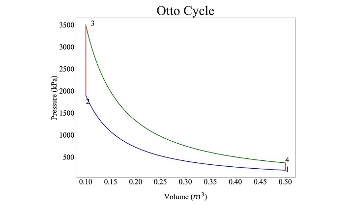
The pressures and volumes at different points obtained from the code is as follows −

State	p	v
1	2.000000e+05	0.5
2	1.903654e+06	0.1
3	3.500000e+06	0.1
4	3.677139e+05	0.5

Diesel Cycle

An air standard cycle used in compression ignition (CI) engines is the diesel cycle. Four processes make up the cycle − two reversible adiabatic, one isobaric (constant pressure), and two isochoric (constant volume). Heat addition happens in process 2-3, whereas heat rejection happens in process 4-1. The processes 1-2 and 3-4, respectively, are where the work interaction to and from the cycle takes place. The Diesel cycle diagram is shown in Figure given below.

To model the cycle, the input variables considered are maximum pressure $\mathrm{(p_{max})}$, minimum pressure $\mathrm{(p_{min})}$, maximum volume $\mathrm{(v_{max})}$, cut-off ratio $\mathrm{(r_{c})}$, and adiabatic exponent \mathrm{(\gamma)}. The thermodynamic computations of different processes involved in the Diesel cycle are explained below −

Process 1-2

$$\mathrm{p_{1} \: = \: p_{min}}$$

$$\mathrm{v_{1} \: = \: v_{max}}$$

$$\mathrm{p_{2} \: = \: p_{max}}$$

Since 1-2 is an adiabatic process, so it follows $\mathrm{pv^{\gamma} \: = \: const \: ;}$ let the constant be $\mathrm{(c_{1})}$. The volume at point 2 can be evaluated as −

$$\mathrm{v_{2} \: = \: v_{1} \: \times (\frac{p_{1}}{p_{2}})^{\frac{1}{\gamma}}}$$

Therefore $\mathrm{c_{1} \: = \: p_{1} \: \times \: v_{1}^{\gamma}}$

Then the adiabatic constant along the process 1-2 is evaluated as −

$$\mathrm{c_{1} \: = \: p_{1} \: \times \: v_{1}^{\gamma}}$$

Once $\mathrm{c_{1}}$ is known, the pressure variation along the line 1-2 is evaluated as −

$$\mathrm{p \: = \: \frac{c_{1}}{v^{\gamma}}}$$

Process 2-3

As the process is isobaric, so the pressure remains the same, thus −

$$\mathrm{p_{3} \: = \: p_{2}}$$

The volume at point 3 can be evaluated as −

$$\mathrm{v_{3} \: = \: r_{c} \: \times \: v_{2}}$$

So, the pressure variation between volumes $\mathrm{v_{2}}$ and $\mathrm{v_{3}}$ can be known easily.

Process 3-4

Let $\mathrm{c_{2}}$ be the constant along line 3-4. As pressure and temperature at point 3 are known, so the constant along the reversible adiabatic line can be evaluated as −

$$\mathrm{c_{2} \: = \: p_{3} \: \times \: v_{3}^{\gamma}}$$

And as $\mathrm{v_{4} \: = \: v_{1}}$, so the pressure variation along 3-4 can be evaluated as −

$$\mathrm{p \: = \: \frac{c_{2}}{v^{\gamma}}}$$

Process 4-1

$\mathrm{c_{2}}$ and $\mathrm{v_{4}}$ are already known, so $\mathrm{p_{4}}$ can be evaluated as

$$\mathrm{p_{4} \: = \: \frac{c_{4}}{v^{\gamma}_{4}}}$$

Python Program to Model the Diesel Cycle

The python function to model the Diesel cycle is as follows −

#~~~~~~~~~~~~~~~~~~~
# Diesel Cycle
#~~~~~~~~~~~~~~~~~~~
   def diesel(p_min,p_max,v_max,r_c,gma):
   font = {'family' : 'Times New Roman','size' : 39}
   figure(figsize=(20,15))
   title('Rankine Cycle with Feed water heating (T-s Diagram)',color='b')
   rc('font', **font)
   '''This function prints Diesel cycle
   arguments are as follows:
   p_min: minimum pressure
   p_max: Maximum pressure
   v_max: Maximum volume
   rc: Cut-Off ratio
   gma: Adiabatic exponent
   The order of arguments is:
   p_min,p_max,v_max,rc,gma
   '''

#~~~~~~~~~~~~~~~~~~~~~~~~~
# Process 1-2
#~~~~~~~~~~~~~~~~~~~~~~~~~
   p1=p_min
   v1=v_max
   p2=p_max
   v2=v1*(p1/p2)**(1/gma)
   c1=p1*v1**gma
   v=linspace(v2,v1,100)
   p=c1/v**gma
   plot(v,p/1000,'b',linewidth=3)
   
#~~~~~~~~~~~~~~~~~~~~~~~~~
# Process 2-3
#~~~~~~~~~~~~~~~~~~~~~~~~~
   p3=p2
   p=zeros(100)
   p=p+p2
   v3=r_c*v2
   v=linspace(v2,v3,100)
   plot(v,p/1000.,'r',linewidth=3)
   
#~~~~~~~~~~~~~~~~~~~~~~~~~
# Process 3-4
#~~~~~~~~~~~~~~~~~~~~~~~~~
   v4=v1
   c2=p3*v3**gma
   v=linspace(v3,v4,100)
   p=c2/v**gma
   plot(v,p/1000,'g',linewidth=3)
   
#~~~~~~~~~~~~~~~~~~~~~~~~~
# Process 4-1
#~~~~~~~~~~~~~~~~~~~~~~~~~
   v4=v1
   v=100*[v4]
   p4=c2/v4**gma
   p=linspace(p1,p4,100)
   plot(v,p/1000.,'m',linewidth=3)
   title('Diesel Cycle',size='xx-large',color='b')
   xlabel('Volume ($m^3$)')
   ylabel('Pressure (kPa)')
   text(v1,p1/1000-30,'1')
   text(v2-0.01,p2/1000,'2')
   text(v3+0.01,p3/1000-20,'3')
   text(v4,p4/1000+10,'4')
   data={'p':[p1,p2,p3,p4],
      'v':[v1,v2,v3,v4],
      'c':[c1,'' ,c2,'' ],
      'State': [1,2,3,4]}
   df=DataFrame(data)
   savefig('Diesel_final.jpg')
   return df.set_index('State')
   dc=diesel(2*10**5,20*10**5,0.5,2,1.4)
   show()
   dc

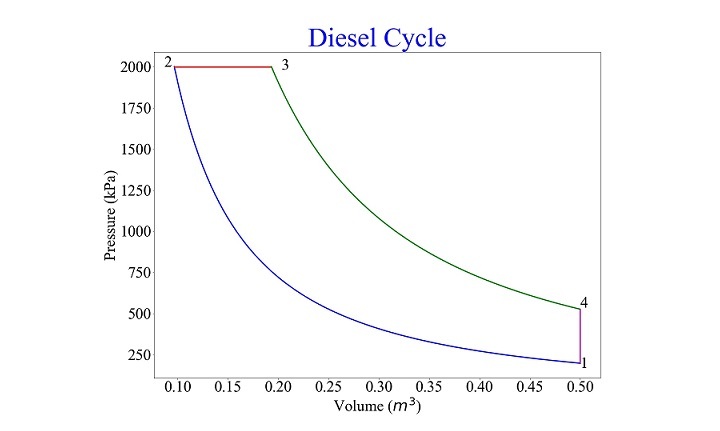
For $\mathrm{p_{min} \: = \: 2 \: \times \: 10^{5} \: Pa \: , \: p_{max} \: = \: 20 \: \times \: 10^{5} \: Pa \: , \: v_{max} \: = \: 0.5 \: m^{3} \: , \: r_{c} \: = \: 2 \: and \: \gamma \: = \: 1.4 \: ,}$ the results obtained are shown in Figures given below

State	p	v
1	2.000000e+05	0.500000
2	2.000000e+06	0.096535
3	2.000000e+06	0.193070
4	5.278032e+05	0.500000

Conclusion

In this tutorial, the Otto and Diesel cycles are modelled with the help of Python Programming. Function of Diesel and Otto cycles were Programmed and tested. The function is capable to draw the cycles based on the input data.