How to hide formula not displayed in the formula bar in Excel?

Excel has a setting that prevents the software from showing formula outcomes. In clearer terms hiding an active sheet formula is possible. If the user inputs a formula into an empty cell with text formatting, the result will never appear. One can use formulas in a worksheet to advantage, and they are typically shown in the Formula bar. However, if there are any essential numbers that the user does not want to disclose with other than this option seems to be very useful. As it will allow the user to hide the way to process the provided data.

Example 1: To hide the formula associated with any column in the formula bar of an Excel

Step 1

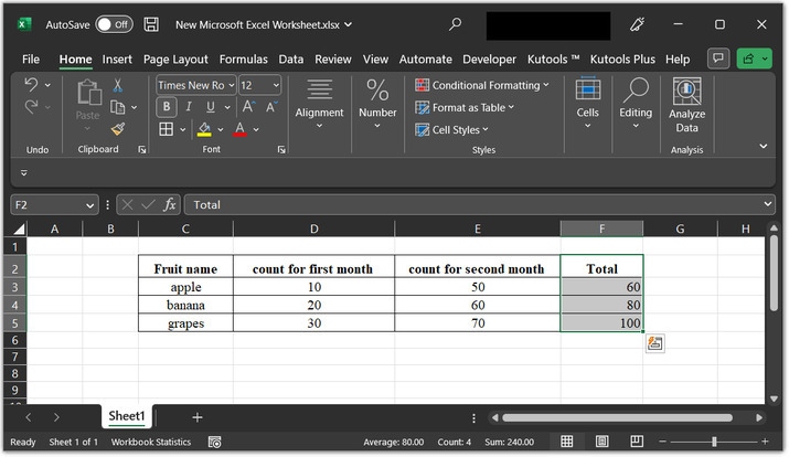
To understand the process of hiding the formula, by using the format cell feature. Consider the below-provided sample worksheet. This worksheet contains, a total of 4 columns, the first column contains the fruit name, and the second and third column contains an available count for first and second-column values. The total columns contain data for the second and third columns. The sum can easily see from the formula tab.

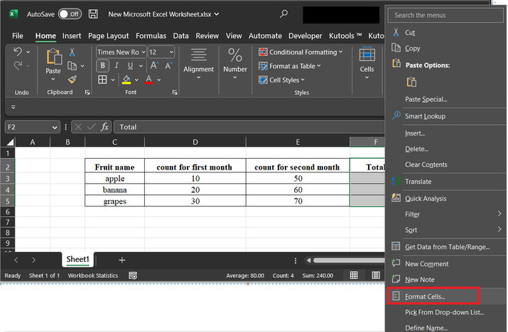
Step 2

After that select the range and use right click to obtain the required feature. This will display the list of options. From the provided list of options select the “Format Cells..”.

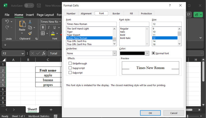
Step 3

The above step will open a “Format Cells” dialog box. This dialog box contains many tabs such as numbers, alignment, and many others. The reference image for the dialog box can be seen below −

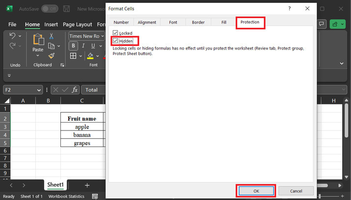
Step 4

Go to Protection Tab in the dialog box named Format Cells and select the Hidden check box option. This option will hide the formula used with the selected data column. Finally, click on the “OK” button.

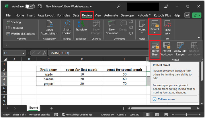
Step 5

After clicking on the “Review” Tab. Go to the “Protect” section, and then click on the “Protect Sheet” option.

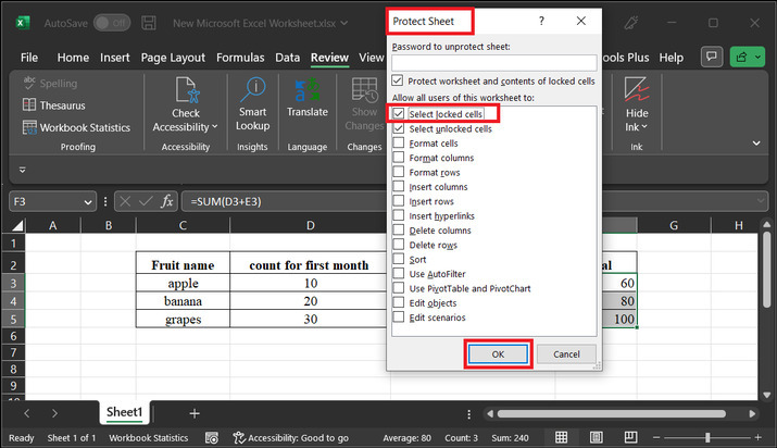
Step 6

And then the “Protect Sheet” dialog box would be open. In this dialog box, tick the option for “Select locked cells” and finally click on the “OK” button.

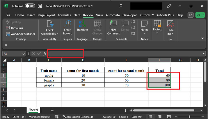
Step 7

After that go to the Excel sheet and select the cell F3 to F6, as given below. Observe the highlighted formula area, this time formula is not visible in the formula bar.

Conclusion

After learning all the guided steps carefully, the learner will be able to hide the formula of any column easily. Please note that the same approach can be used for more than one column, the only required thing is that the user needs to select the column, again and need to enable the “hide” option. In more simple terms, the process involves the repetition of the same guided step for all the number of columns, which requires locking their formula.

For example, if two columns want to lock their formula, then the same process can be done twice. This article contains a thorough explanation of all the required steps. The provided task can be done accurately with the help of the illustrated steps.