
Article Categories
- All Categories
-
 Data Structure
-
 Networking
-
 RDBMS
RDBMS
-
 Operating System
-
 Java
Java
-
 MS Excel
-
 iOS
iOS
-
 HTML
HTML
-
 CSS
CSS
-
 Android
-
 Python
-
 C Programming
-
 C++
C++
-
 C#
C#
-
 MongoDB
-
 MySQL
MySQL
-
 Javascript
-
 PHP
PHP
-
 Economics & Finance
How to Lock and Protect Selected Cells in Excel?
In this article, the user will learn the process of locking and protecting some selected cells in Excel. Locking and protecting nonempty cells in a selected range with the "Protect Sheet" feature in spreadsheet applications like Excel or Google Sheets provides an additional layer of security to prevent accidental or unauthorized modifications to important data.
By using the "Protect Sheet" feature and locking selected cells, the user can add an extra level of control and safeguard to the user spreadsheet, promoting data integrity, collaboration, and data security. In this article, two examples are provided. The first example, allow the user to lock and protect the selected cell, in the selected range, by using the available Excel features, and option. While the second example allows user to understand the process of using the kutools tools to lock and protect the cell data.
Example 1: To Lock and protect selected cells in a selected range with Protect Sheet
Step 1
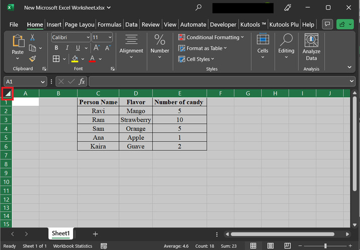
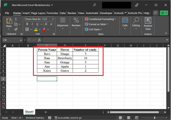
To understand the process of locking and protecting selecting cells, the user first needs to consider a sample table, as shown below. In the below-given table, will be using three columns named Person Name, Flavor, and Number of candy. In this example will select all cells, to do so click on the right-angle triangle symbol provided at the top of the left-hand side, consider the below-given sheet for proper reference:
Step 2
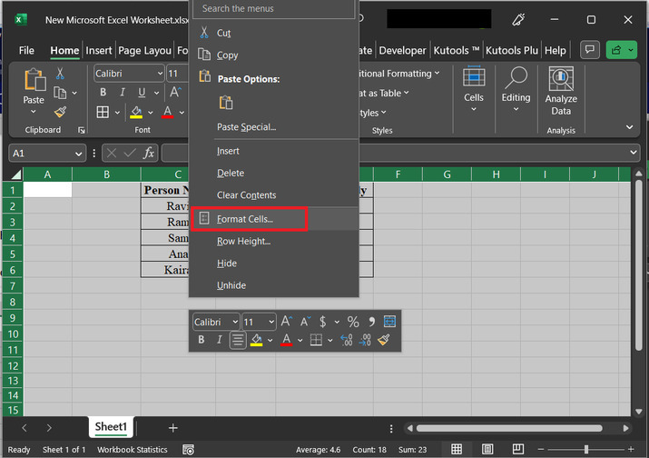
The above step will select all the available cells, as shown below. After that right click on any of the selected cells. This will display a list of available options. Among the displayed list of options, select the option with "Format Cells".
Step 3
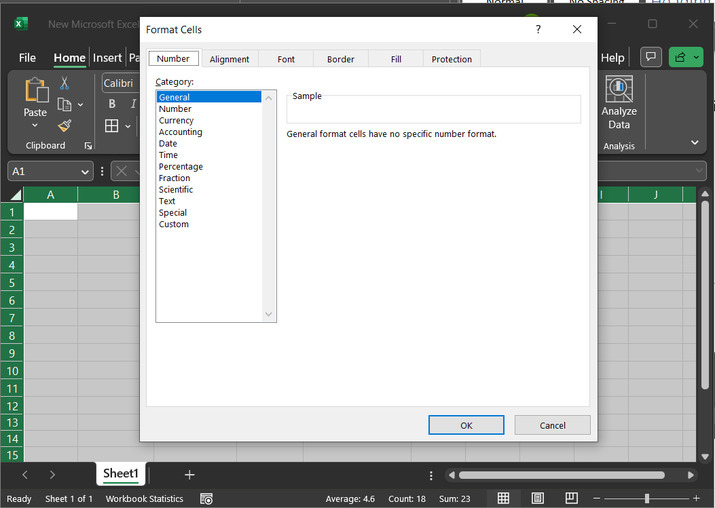
The above step will display a dialog box for "Format cells". This option will display multiple tabs, here each tab has multiple options. Consider below given image snapshot for proper reference:
Step 4
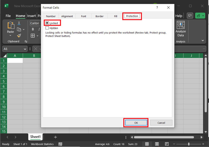
Among all the available tabs, choose the "Protection" tab, and untick the "Locked" option. Finally, click on the "OK" button.
Step 5
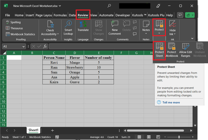
In the review tab, click on the "Protect" tab, and select the option for "Protect Sheet". Consider the below depicted image for reference:
Step 6
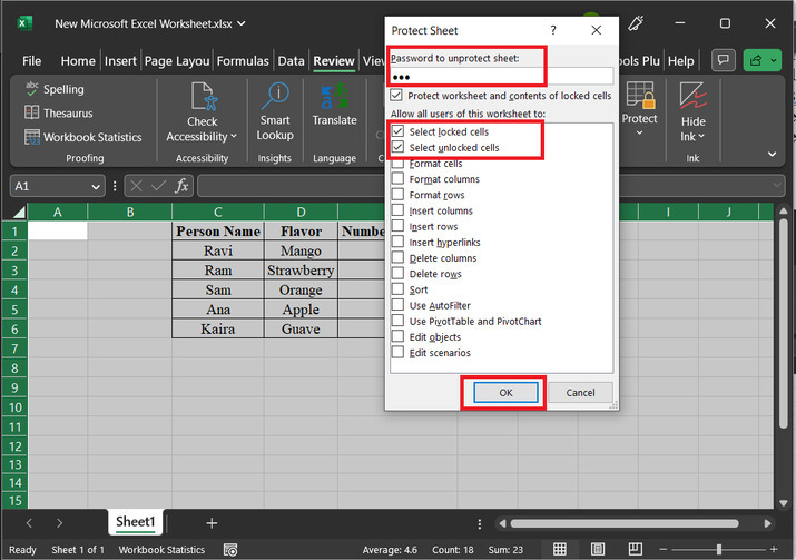
The above step will open a new dialog box, with the header "Protect Sheet". In this dialog box, first, enter the password to make the sheet unprotected. In this example will assume that the password is "abc". Please note that users can use any desirable password. But, make sure to remind the user password, as to make any change or to unprotect the sheet, the user needs this password only. After that select both first two options "Select locked cells" and "Select unlocked cells". Finally, click on the "OK" button.

Step 7
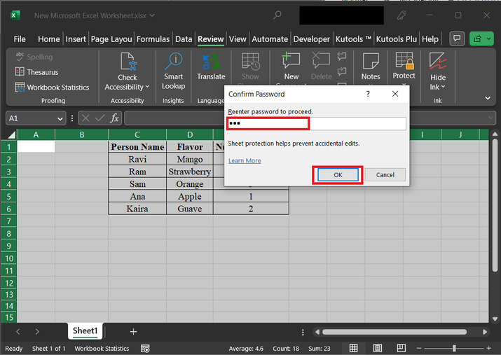
This will open a "Confirm Password" dialog box. This dialog box will allow the user to enter the password again, and click on the "OK" button.
Step 8
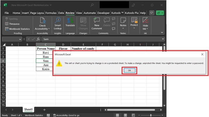
After that, try to click and edit any cell. in this example, the user is trying to modify the contents of the C4, cell. But this will display a dialog box, with the message, as depicted below. To remove the error message, click on the "OK" button.
Example 2: To Lock and protect selected cells from editing by using the kutools in excel.
Step 1
To understand the process of locking and protecting selecting cells, the user first needs to consider a sample table, as shown below. In the below given table, will be using three columns. The first column contains the person's name, the second column contains the favorite flavor and the final third column contains the number of candy.
Step 2
In this example will select all cells, to do so click on the right-angle triangle symbol provided at the top of the left-hand side. This step will select all the available cells. Consider the below given sheet for proper reference:

Step 3
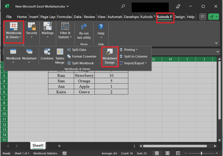
After that go to the "Kutools Plus" tab, and then click on "Workbooks & Sheets". Further, click on "Worksheet Design". Consider the below given image for reference:
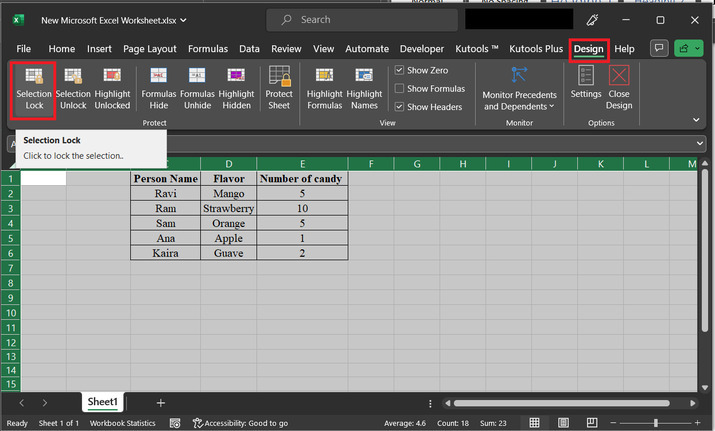
Step 4
The above step will open a "Design" tab. After that click on the "Selection Lock" option. Consider the below depicted image for reference:
Step 5
The above step will ultimately display the message dialog box, as shown below:
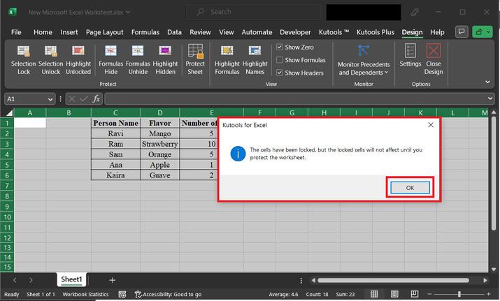
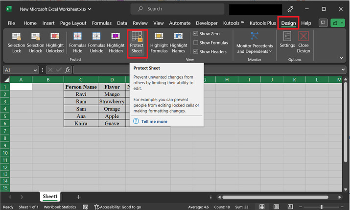
Step 6
Simply click on the "OK" button, as Select the "Protect Sheet" option, as specified below:
Step 7
The above step will open a new dialog box, with the header "Protect Sheet". In this dialog box, first, enter the password to make the sheet unprotected. In this example will assume that the password is "abc". Please note that users can use any desirable password. But, make sure to remind the user password, as to make any change or to unprotect the sheet, the user needs this password only. After that select both first two options "Select locked cells" and "Select unlocked cells". Finally, click on the "OK" button.
Step 9
This will open a "Confirm Password" dialog box. This dialog box will allow the user to enter the password again and click on the "OK" button.

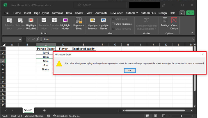
Step 10
After that, try to click and edit any cell. in this example, the user is trying to modify the contents of the C4, cell. But this will display a dialog box, with the message, as depicted below. To remove the error message, click on the "OK" button.
Conclusion
In this article, the user will learn the process of locking and protecting the selected cells of the Excel sheet. This article briefs the same task with two different approaches, although the output of both examples is the same. As, two different approaches, shows that a single task can be done in more than one way. All the provided steps are clear, precise, thorough, and fully relevant to the provided content.

460 Views
