How to group data by half a year in Excel pivot table?

In this article, users will understand how to group data by half a year in an Excel pivot table. A pivot table is an excellent option presented in MS Excel to interpret and summarize the large voluminous of data. This article contains an example that uses the pivot table option available in the insert table, to group the available year data of an Excel pivot table. In the initial steps, the table is converted into a pivot table, and further, the obtained table data is grouped according to the user's requirement.

Example 1: To group a pivot table by half year in Excel by using the pivot table option

Step 1

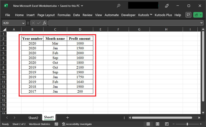
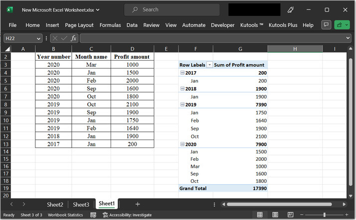
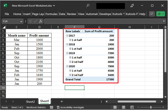
To understand the processing of data by half a year in excel pivot table, consider the below given excel sheet. This sheet contains three columns. The first column contains data for year number, second column contains data for month name, and third column contains the column for profit amount.

Step 2

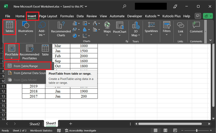
In this step, the user needs to first create a pivot table. To create a pivot table go to the “Insert” tab, click on the “Tables” option, then choose the option for “Pivot Table”, and click on the first available option, “From Table/ Range”. To understand the chosen options more precisely refer to the snapshot provided below −

Step 3

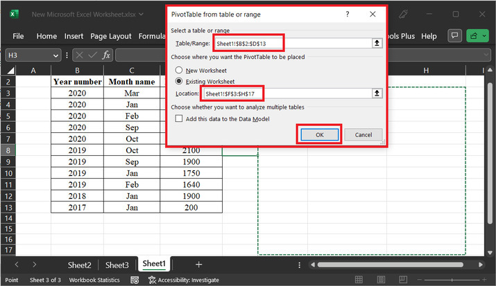
The above step will display a dialog box for “PivotTable from table or range”. In the table/range label, select the table data already provided in the Excel sheet. From the two provided radio buttons, select the second option, which contains the location of the sheet, and click on the “OK” button.

Step 4

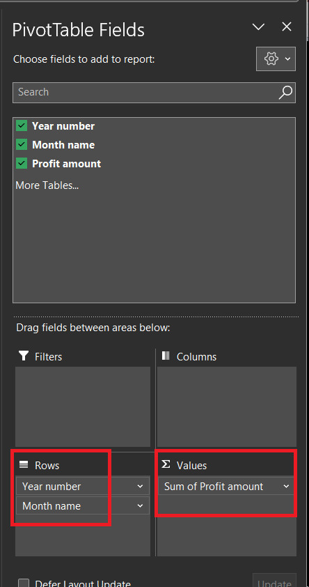
The above step will open a dialog box for “PivotTable Fields”. In this dialog box, all the column values are listed in the choose field option. In the rows, the section opens the option for “Year number”, and “Month name”, and in the values column, drag and drop the column profit amount.

Step 5

The above step will ultimately create the below-given pivot table.

Step 6

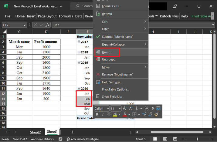
Before moving further remember that in this task user needs to group half-year months. This means that a year has a total of 12 months so, will consider the first 6 months and group them as Group 1, and similarly, the rest 6 months can be listed in the second group. To do so, select the first 6 months together, and click on the group option. After that select the last 6 months and right-click on the option to group them in group 2.

Step 7

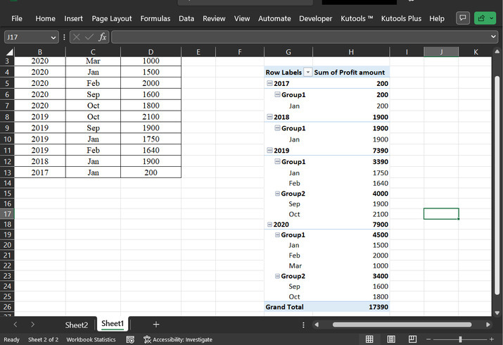
After the completion of the above step, the first 6 months of the year that is Jan, Feb, Mar, Apr, May, and June will be displayed in group 1, while the rest 6 months of the year will be displayed in group 2. This will modify the table and data will be displayed in the form of a group as shown below −

Step 8

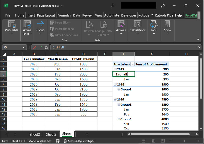
Now, let’s rename the group. To do so, click on the group name, and enter 1st half to group 1 −

Step 9

Perform the same for 2nd half of group 2. After modification of the group name, the label data will appear as given below −

Conclusion

After going through all the provided steps, the user will be able to generate a pivot table from the provided normal table in Excel and can also be able to group the data into half a year by using separate groups. This example describes a simple way to solve the required task. It is very important to note that by referring to the article precisely the user can perform other possible similar tasks as well, such as grouping data in product categories and many others.