How to group date by month, year, half year or other specific dates in Excel pivot table?

Grouping the data in Excel Pivot Table is a way to group numerical data into specific categories such as month, year, half year, and many others. This feature allows the user to summarize and analyze data based on different ranges of values, instead of individual values. This article contains a single example that uses the pivot table option available in the insert table, to group the available year data of an Excel pivot table. This article will first provide a normal Excel table. In the initial steps the table is converted into a pivot table, and further, the obtained table data is grouped according to the user requirement −

Example 1: To group a pivot table date by month, year, and half year in Excel by using the pivot table option

Step 1

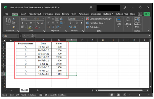
To understand the process of grouping dates by year, month, or year. Users first need to create a table, and then map the table to a pivot table, further group the pivot table to display the data accordingly. Create a table with 3 columns, the first column contain data for product name, the second column contains data for date, and the third column contains data records for sales. To understand more precisely consider below given table data −

Step 2

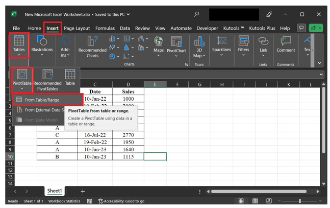
To create a pivot table, go to the “Insert” tab, and then click on the “Tables” option, further select the “Pivot Table” option, and then click on the option “Pivot Table”. Further select the option for “From Table/Range”.

Step 3

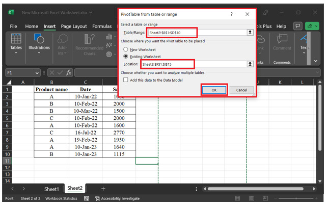
The above step will open a “Pivot Table from table or range” dialog box. In this dialog box. In the table/range dialog box, select the available table, to add the data fields for a new pivot table. Select the option “Existing Worksheet”. Under the location tag, select the new location for a pivot table. Finally, click on the “OK” button.

Step 4

The above step will open a “Pivot Table Fields” dialog box. This dialog box contains all the selected fields. Drag the date field to the rows section, and the sales sum to the sum value column header. Consider the below-given image for reference −

Step 5

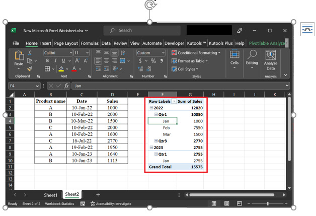
The above step will display the pivot table given below −

Step 6

Click on the available plus sign to display the pivot table record values −

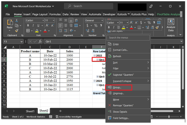
Step 7

After that select any data field, and use right click. This will display a list of multiple options. Among the list of displayed options, select the option named “Group”.

Step 8

This will display a “grouping” dialog box, as given below. In the appeared dialog box, enter the values for the “Starting at”, and “Ending at” labels, according to the provided details, and select the required appropriate option. Finally, click on the “OK” option.

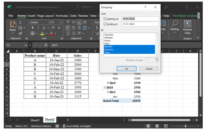
Please note that the chosen step will modify the output tables accordingly.

Conclusion

After going through all the provided steps, the user will be able to generate a pivot table from the provided normal table in Excel and can also be able to group the data into half years, quarters, or months by using separate groups. This example describes a simple way to solve the required task. It is very important to note that by referring to the article precisely the user can perform other possible similar tasks as well, such as grouping the data into different time categories.