
Article Categories
- All Categories
-
 Data Structure
-
 Networking
-
 RDBMS
RDBMS
-
 Operating System
-
 Java
Java
-
 MS Excel
-
 iOS
iOS
-
 HTML
HTML
-
 CSS
CSS
-
 Android
-
 Python
-
 C Programming
-
 C++
C++
-
 C#
C#
-
 MongoDB
-
 MySQL
MySQL
-
 Javascript
-
 PHP
PHP
-
 Economics & Finance
How To Display Table Or Pivot Table Name In A Cell In Excel?
Powerful spreadsheet programmes like Excel provide a variety of features for arranging, processing, and displaying data. Making tables and pivot tables, which make it simple to summarise and work with big amounts of data, is a useful tool.
It can be useful to list the names of the tables or pivot tables in a cell when using several tables or pivot tables in Excel for documentation or reference. When dealing with complicated spreadsheets, you can easily determine the data source or analysis being used by doing this.
We'll walk you through how to display table or pivot table names in an Excel cell in this tutorial. This step?by?step manual will show you how to use this tool to improve your data management and analysis workflows, regardless of your level of experience.
Display Table Or Pivot Table Name In A Cell
Here we will first create a user?defined formula using the VBA application and then use the formula to complete the task. So let us see a simple process to know how you can display a table or pivot table name in a cell in Excel.
Step 1
Consider an Excel sheet where you have a pivot table or something similar to the below image.
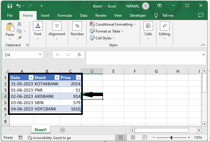
First, right?click on the sheet name and select View Code to open the VBA application, then click on Insert and select Module.
Right click > View code > Insert > Module.
Step 2
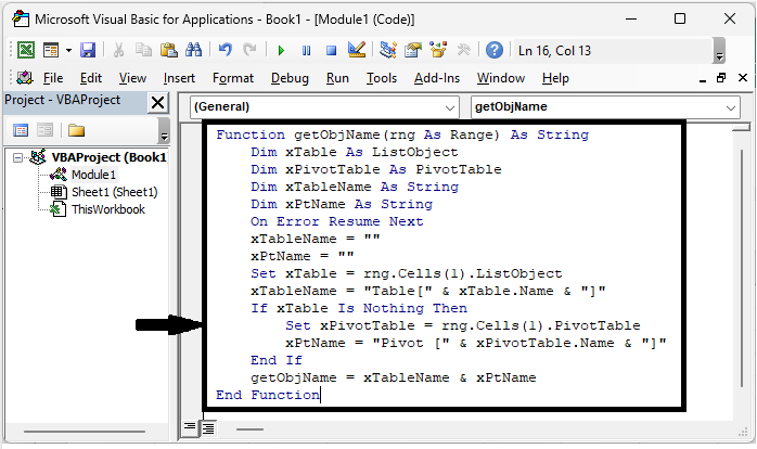
Then copy the below code into the text box.
Code
Function getObjName(rng As Range) As String
   Dim xTable As ListObject
   Dim xPivotTable As PivotTable
   Dim xTableName As String
   Dim xPtName As String
   On Error Resume Next
   xTableName = ""
   xPtName = ""
   Set xTable = rng.Cells(1).ListObject
   xTableName = "Table[" & xTable.Name & "]"
   If xTable Is Nothing Then
      Set xPivotTable = rng.Cells(1).PivotTable
      xPtName = "Pivot [" & xPivotTable.Name & "]"
   End If
   getObjName = xTableName & xPtName
End Function
Step 3
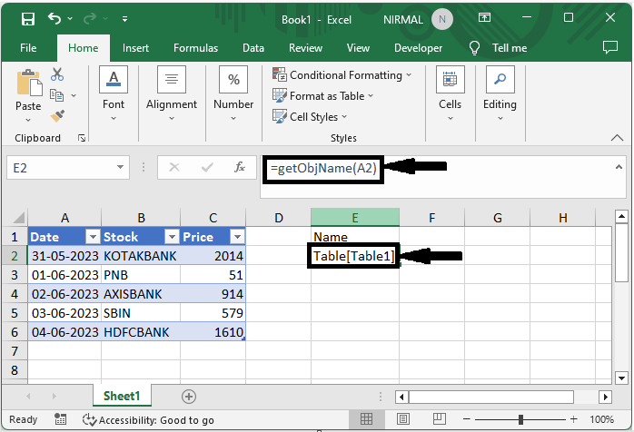
Then close the VBA using ALT + Q. then click on an empty cell and enter the formula as =getObjName(A2) and click enter to complete the task. Here, A2 is the address of any cell in the table.
Close > Empty cell > Formula > Enter.
Conclusion
In this tutorial, we have used a simple example to demonstrate how you can display a table or pivot table name in a cell in Excel to highlight a particular set of data.

2K+ Views
