How to group by week in pivot table?

A pivot table is an essential tool present in MS Excel that rapidly analyzes and summarizes large voluminous of data in a table format. Grouping data by week usually means that the provided data is categorized by using week. This article covers three examples, first two examples are using the same strategy with a day or period difference of a week. But, in the last example, use a helper column to perform the same task, this helper column can be manipulated with the help of provided column.

Example 1: To group the week in the pivot table by using 7 day or single period week

Step 1

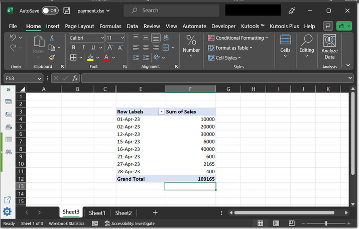
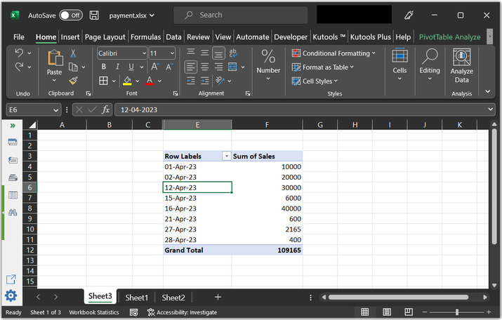
To understand the process of grouping provided a date by a week, using the 7-day concept. Consider below given pivot table −

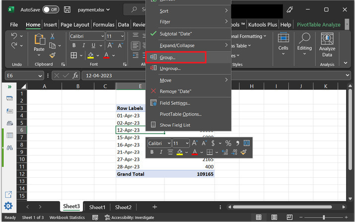
Step 2

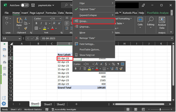
Go to the table and right-click on any date available in the table. This will open a menu bar with multiple options. Select the option “Group…”. Consider the below-given image for reference −

Step 3

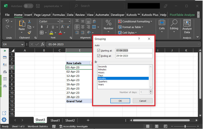
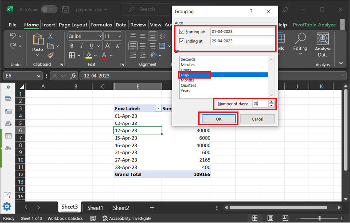
This will open the “Grouping” dialog box. This dialog box contains many fields. Under the “Auto” category user can set the starting date under the “Starting at” input label, and secondly under the end date user can set the end data under the “Ending at” option. Under the “by” option list user can set the option according to the requirement.

Step 4

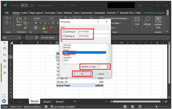
Users can manually enter data into both the provided field if required. But, for this example, the data range is already selected, and the displayed date is accurate. So, there is no need to modify the provided date. However, if the user wants, then changing data is possible. Move to the next header “by”. Since, in the example, the user wants to create 7 days. Thus, select the “Days” option. Now, go down and the “Number of days” option is found, then select “7”. Click on “OK”. Consider the below-depicted image for proper reference −

Step 5

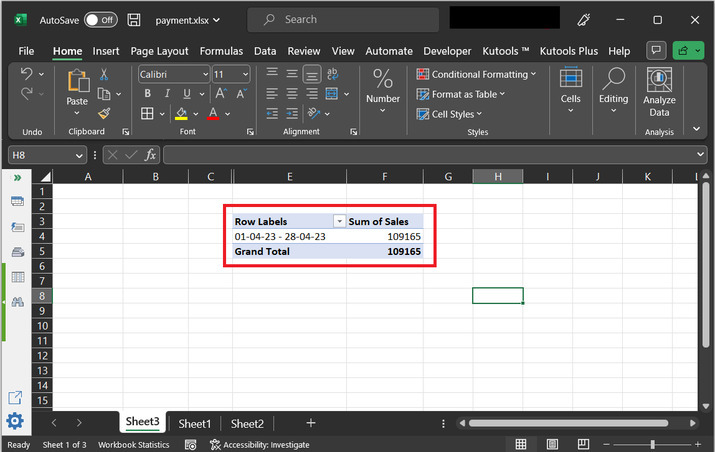
This will display the given data as a 1-week range. Consider the results provided in the below snapshot −

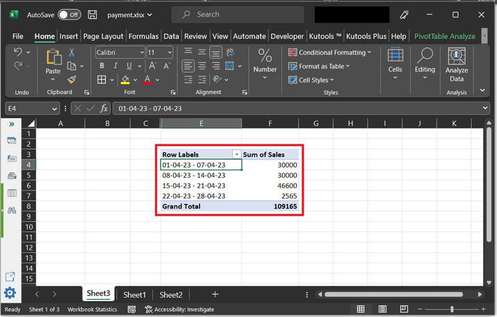
Example 2: To group the week in pivot table by using the 4-period week concept

Step 1

Group four weeks in a pivot table. Consider the below-given spreadsheet, and right-click on the date column.

Step 2

Select the “Group” option. As shown below −

Step 3

This will open the “Grouping” dialog box, and then select the Starting at, and Ending at date accordingly. In the by section select “Days”. Set the Number of days as “28”, and press “OK”.

Step 4

The above step will provide a consolidated data of 4 weeks.

Example 3: To group the week in the pivot table by using the helper column

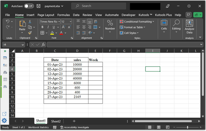
Step 1

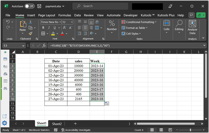
Consider the below given below spreadsheet. The below given worksheet contains the date, sales, and week column.

Step 2

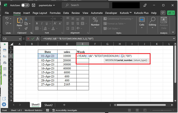
Go to the E3 cell, and type the formula

“=YEAR(C3)&" "&TEXT(WEEKNUM(C3,2),"00")” and press “Enter” key.

Explanation

• YEAR(C3) returns the year value of the date in cell C3.

• "&" is used for concatenation.

• "-" is a string literal that will be included in the concatenated text.

TEXT(WEEKNUM(C3,2),"00") returns the week number of the date in cell C3, with the second argument specifying that the week starts on Monday. The "00" format code ensures that the week number is displayed with two digits.

Put all these together with the "&" concatenation operator. Getting a text string that represents the year and week number of the date in cell C3 in the format of "YYYY-WW", where YYYY is the four-digit year value and WW is the two-digit week number.

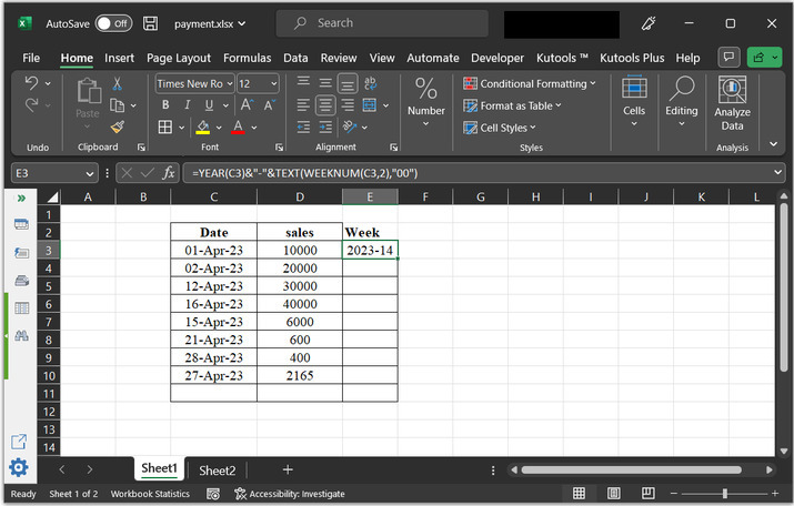
Step 3

The results are displayed below −

Step 4

Click on the plus “+” sign at the bottom of the cell and then drag the cell to the 10 rows, to copy the same formula for all the available cells.

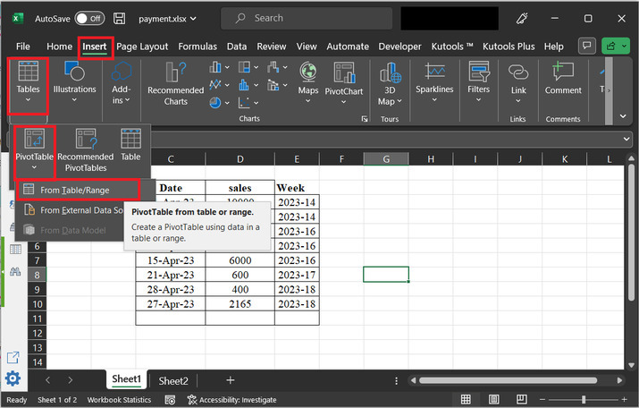
Step 5

After that go to the “Insert” tab, and then select the option “Tables” option, select the option “Pivot Table”, then select “From Table/Range”.

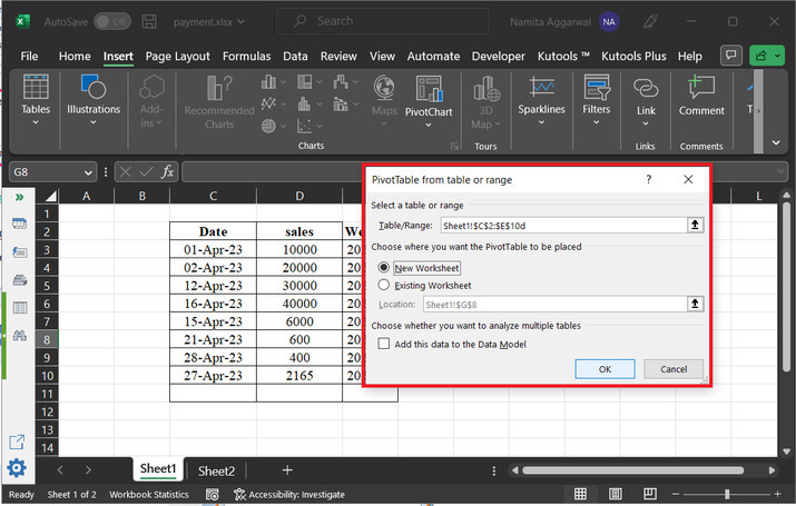
Step 6

This will open the “PivotTable from table or range” dialog box. In the open dialog select the available table range. And in the “choose where you want the PivotTable to be placed” label, select the option “New worksheet”. Finally, click on the “OK” button.

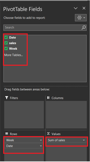
Step 7

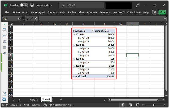
To display the required pivot table on the new worksheet. Select the below-specified values, “date, sales, and week” entries. After that in the rows, section add the week and date. In the values section, add “Sum of sales”, and other required parameters as specified below −

Step 8

Consider the final obtained pivot table structure −

Conclusion

This article briefs users on three ways to group the week's data by using the pivot table in Excel. Two examples allow the user to group the data, while the third example allows the user to use the helper method to process the same data.