
Article Categories
- All Categories
-
 Data Structure
-
 Networking
-
 RDBMS
RDBMS
-
 Operating System
-
 Java
Java
-
 MS Excel
-
 iOS
iOS
-
 HTML
HTML
-
 CSS
CSS
-
 Android
-
 Python
-
 C Programming
-
 C++
C++
-
 C#
C#
-
 MongoDB
-
 MySQL
MySQL
-
 Javascript
-
 PHP
PHP
-
 Economics & Finance
How to alternate row colour in an Excel Pivot Table?
Displaying alternate row colours in a normal table is a very simple process which can be done using the conditional formatting concept but creating alternate row colour in pivot table is simple problem. A pivot table in Excel is an interactive table which helps in quickly summarizing the data. When we want to add alternate row colour in a pivot table is a lengthy and simple problem.so let us see a simple trick to end this problem.
Let us see a simple process to add alternate row colours in an Excel pivot table.
Step 1
Let us consider the table shown in the following screenshot. We need to choose the alternate row colour in this table.
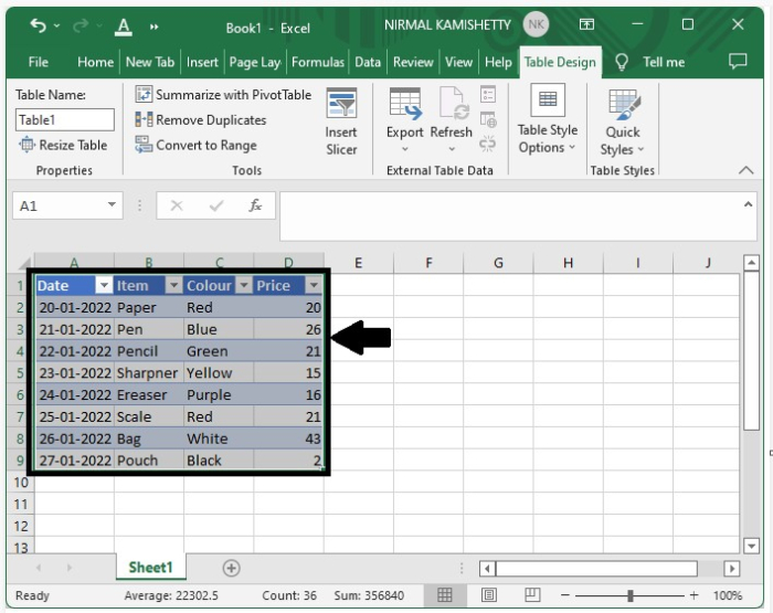
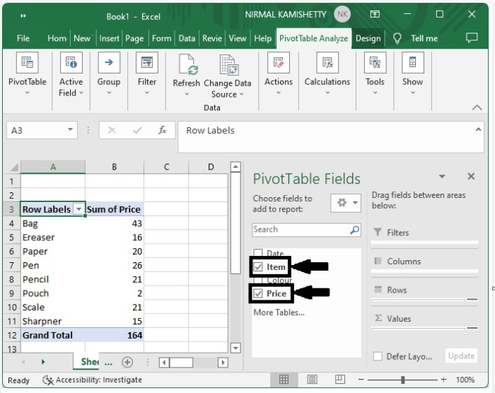
To convert the above table into a Pivot Table, select data >click on insert and select pivot table and choose item and price check boxes and the pivot table will look like the below image.
Step 2
Select the checkbox beside the braided rows under table design.
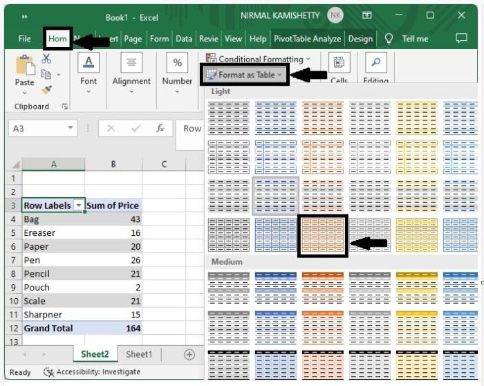
To change the colour of pivot table, click the "Home" tab and select "format table". Then a verity of layouts will appear on the screen; select any one of the styles under the light menu to apply it to the table.
Step 3
After selecting a style in the above step, we will be able to complete our process. The final table will look as shown in the image below ?
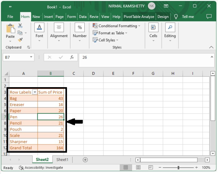
As we can see in the above image, we have successfully completed applying alternate colours in the rows of the pivot table. This is how we can add alternate row colours in an Excel pivot table.

3K+ Views
