How to group time by hour in an Excel pivot table?

Grouping the data in Excel Pivot Table is a way to group numerical data into specific categories such as hours, year, half year, and many others. This feature allows the user to summarize and analyze data based on different ranges of values, instead of individual values. This article contains two examples to demonstrate the provided task. The first example will allow the user to group the pivot table by the hour in Excel. While the second example allows the user to understand the process of grouping the pivot table by hour in Excel.

Example 1: To group a pivot table by the hour in Excel by using the pivot table option

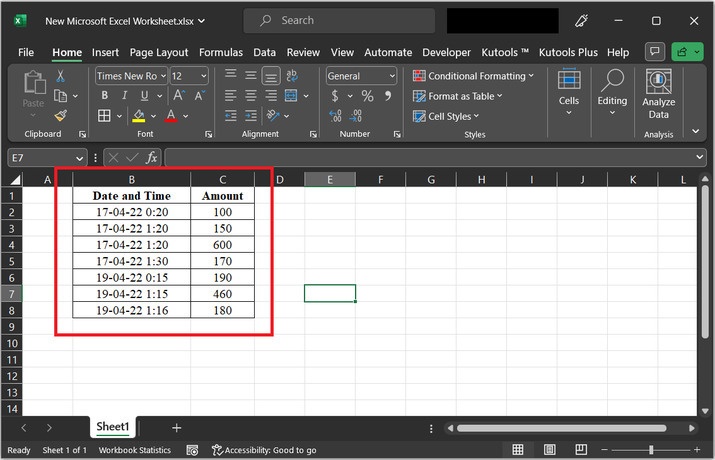
Let’s first create a sample worksheet. In the created table enter the data for date and time and amount. In the date and time column write data for column values. In the second amount column, add data for the amount column.

Step 2

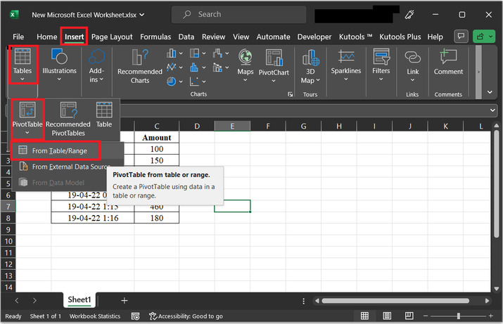
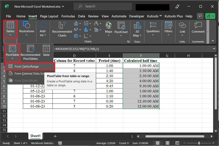
In this step, the user needs to first create a pivot table. To create a pivot table, go to the “Insert” tab, click on the “Tables” option, then choose the option for “PivotTable”, and click on the first available option, “From Table/Range”. To understand the chosen options more precisely refer to the snapshot provided below −

Step 3

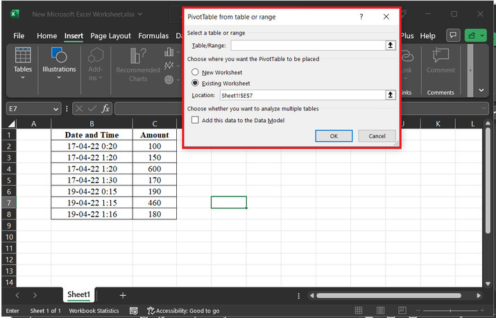
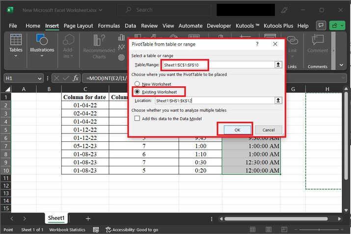
The above step will display a dialog box for “Pivot Table from table or range”. Consider the below given image for reference −

Step 4

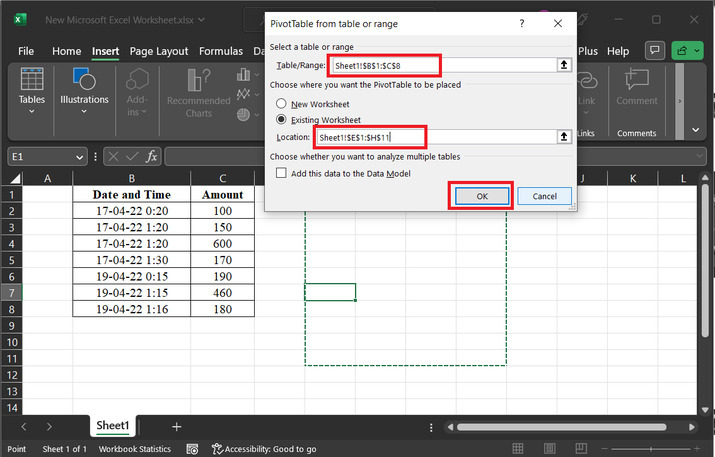
In the table/ range label, add the table data for the provided table, select the radio button for the “Existing Worksheet”, and in the location label, add the location in the table for the area, where the user wants to display the developed pivot table. Finally, click on the “OK” button.

Step 5

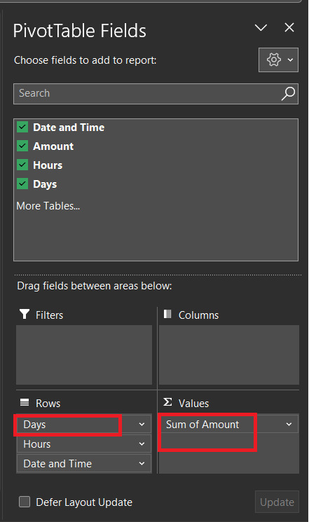
The above step will open a pivot table fields pane. In the opened pane, of the row section drag the data for “date and time”, and in the column section drop the data for the amount value. For proper reference, consider the below-given image −

Step 6

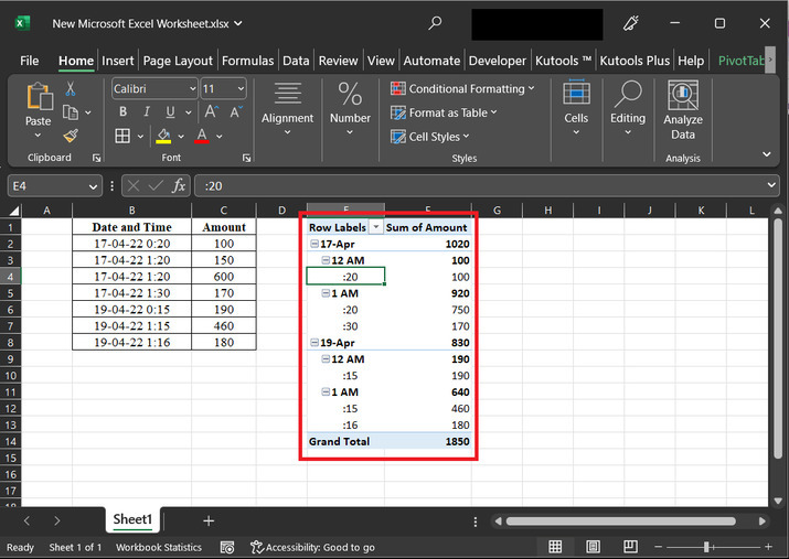
The created pivot table is given below −

Step 7

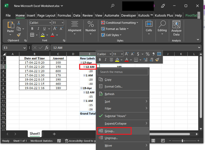
The option will contain a cell value, use right click. This will display the list of available options, as given below −

Step 8

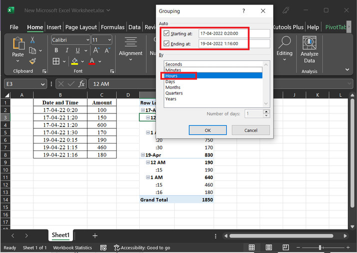
The above step will display a dialog box for “grouping”. Enter the initial date and time in the starting at header, and end date and time in the “ending at” label. In the available by label, select the option for hours. Finally click on the “OK” button.

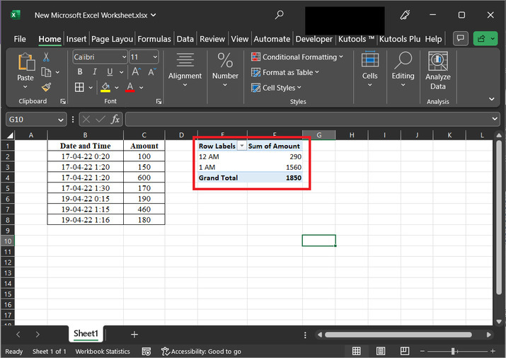
This will display a pivot table, as depicted below −

Example 2: To group a pivot table by half year in excel by using the pivot table option

Step 1

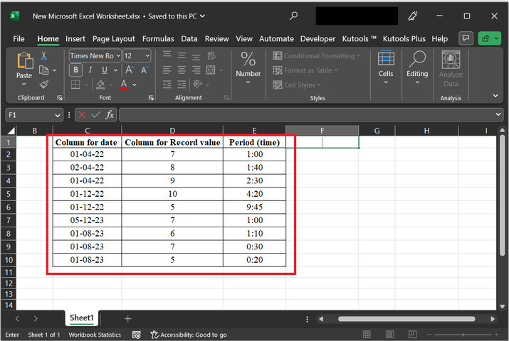
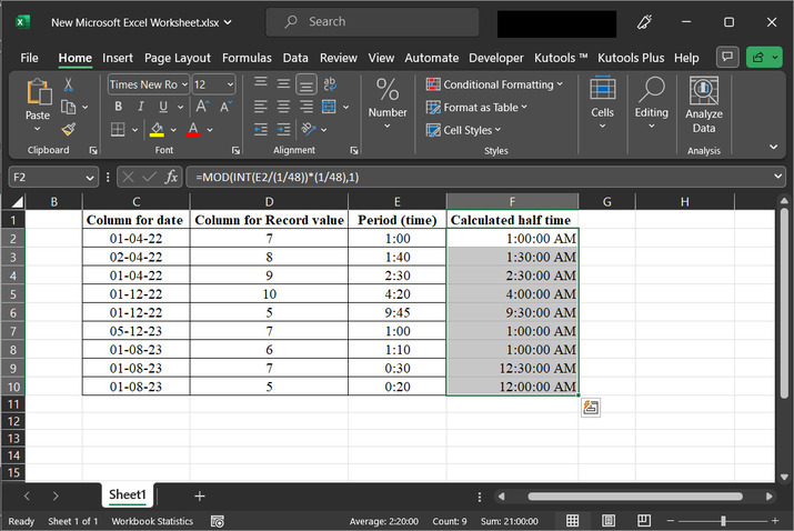
Consider the Excel sheet contains three columns. The first column contains date fields, the second column contains record fields, and the third column contains data fields for the time period. Users can change the cell formatting and syntax according to requirements.

Step 2

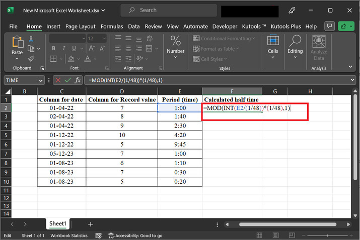
In this step will first create a helper column. To do this, first go to the F2 cell, and then create a column header for the values. By simply writing “calculated half time” to F1 cell. After that go to the F2 cell, and type formula “=MOD(INT(E2/(1/48))*(1/48),1)”. The correct way to do this is described below −

Explanation

• E2− Refers to the value in cell E2.

• 1/48− Represents fraction 1 divided by 48.

• INT(E2/(1/48))− Divides the value in cell E2 by 1/48 and rounds down to the nearest integer.

• (INT(E2/(1/48))*(1/48))− Multiplies the result of above step by 1/48.

• MOD((INT(E2/(1/48))*(1/48)), 1)− Calculates the remainder when dividing the result of the above provided steps.

In summary, the formula calculates the fractional part of the value in cell E2 when divided by 1/48. The result will be a decimal value between 0 and 1

Step 3

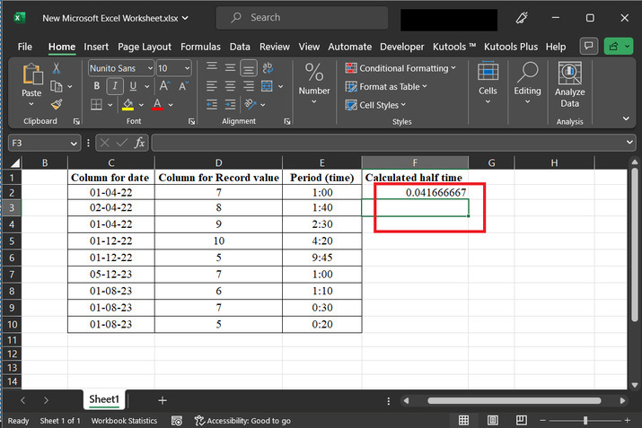
Press “Enter” key to obtain the formula value. The generated result value is 0. Consider the below-provided cell value, as depicted below −

Step 4

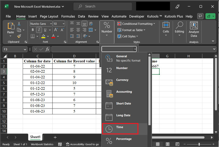
Drag the obtained results to 10, rows, this step will copy the formula for F2 to F10, rows. After the displayed values are shown in the general data type, the user needs to convert the column value to the time data type. To do so, click on the below-provided arrow. This will display the list of options, such as number, currency, and many others. From the provided list of options, select the option with the value, “Time”. Consider below given image snapshot for the proper reference.

Step 5

Drag the F2 cell to F10 cell, this step will copy same formula to different cell values. Now, observe the values of column F, the data appears in the time format. Now, users need to create a separate pivot table to solve the provided task

Step 6

To do so, go to the “Insert” tab, and click on “Tables” option. Among the displayed list of menu options, select the first option for “PivotTable”. After that select the option for “From Table/Range”.

Step 7

The above step will display a “PivotTable from table or range” dialog box, as depicted below. In the appeared dialog box, under the label, table/range select the table data values, and select the option for “Existing Worksheet”. In the location option, the user needs to provide the location where the user wants to place the pivot table. After that click on the “OK” button.

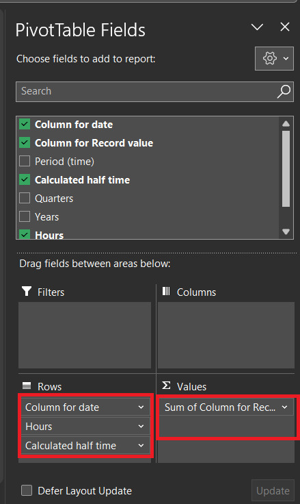
Step 8

The above step will display the dialog box for “Pivot Table Fields”. In the rows section, drag the data values for date and half time. In the values cell column, drag the field data values for the sum of records.

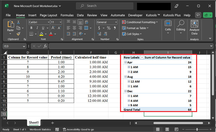
Step 9

The above step will generate a pivot table as given below. This pivot table contains separate header for month name, along with required time, and also displays the sum of records.

Conclusion

In this article, the user will understand the process of grouping time by hour in an Excel pivot table. The two provided examples are simple and contain sufficient explanation to guide the user properly, by referring to this article user will understand the process of working on the pivot table, and grouping the generated table by the hour, half year, and other required groups.