
Article Categories
- All Categories
-
 Data Structure
-
 Networking
-
 RDBMS
RDBMS
-
 Operating System
-
 Java
Java
-
 MS Excel
-
 iOS
iOS
-
 HTML
HTML
-
 CSS
CSS
-
 Android
-
 Python
-
 C Programming
-
 C++
C++
-
 C#
C#
-
 MongoDB
-
 MySQL
MySQL
-
 Javascript
-
 PHP
PHP
-
 Economics & Finance
How To Create A Dynamic Pivot Table To Auto Refresh Expanding Data In Excel?
Welcome to this tutorial on how to create a dynamic Pivot Table in Excel that will automatically refresh as your data expands. Pivot Tables are an incredibly powerful tool in Excel that allow you to analyze and summarize large datasets quickly and easily. However, when working with datasets that are constantly changing or growing, it can be time-consuming to update your Pivot Table manually each time.
In this tutorial, we will show you step-by-step how to create a dynamic Pivot Table that will automatically expand and refresh as new data is added to your dataset. This will save you time and ensure that your analysis is always up-to-date with the latest information. We will walk you through the process of setting up your Pivot Table, creating named ranges, and using Excel's Table feature to ensure that your Pivot Table is always connected to your data source. We will also show you how to use Excel's Power Query tool to clean and transform your data before creating your Pivot Table. By the end of this tutorial, you will have a better understanding of how to create a dynamic Pivot Table in Excel that will save you time and help you make more informed decisions with your data. So, let's get started!
Create A Dynamic Pivot Table To Auto Refresh Expanding Data
Here we will first create a table for the given data, convert the table into a pivot table, and refresh the pivot table after inserting the new data into the table. So let us see a simple process to know how you can create a dynamic pivot table to auto-refresh expanding data in Excel.
Step 1
Consider an Excel sheet where you have data in a table format similar to the below image.
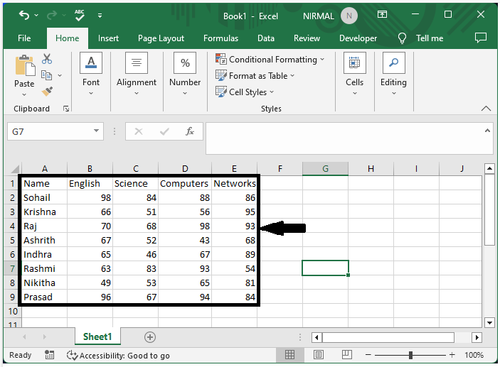
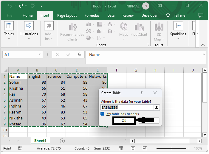
First, select the range of cells, then use the command CTRL + T and click OK to create the table.
Select data > CTRL + T > Ok.
Step 2
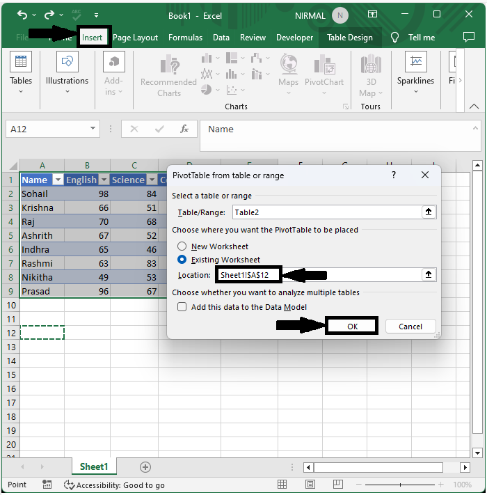
Again, select the table, click on insert, select the pivot table, specify the table location, and click enter.
Select table > Insert > Pivot table > Location > Enter.
Step 3
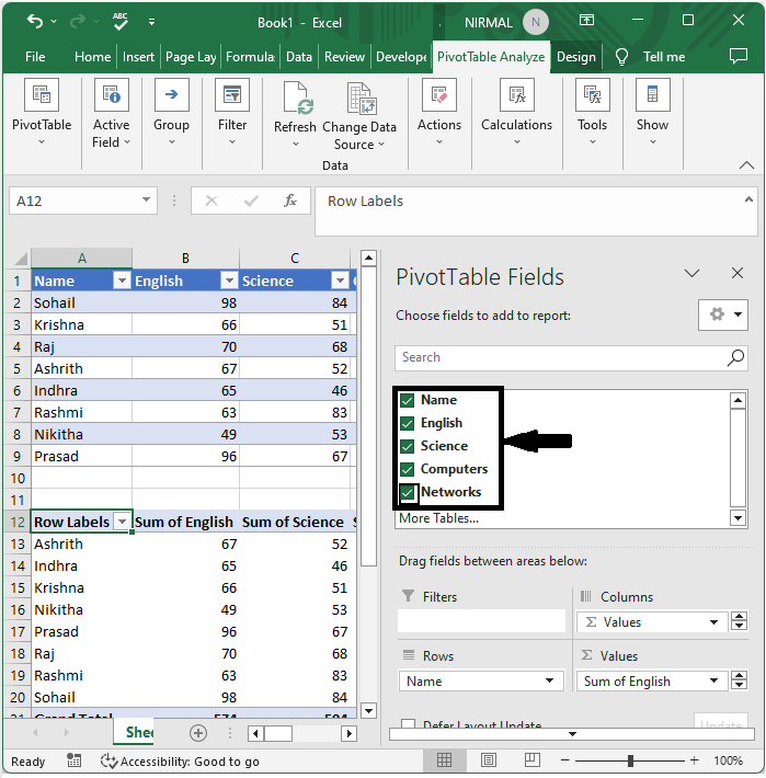
Then select all columns for the pivot table and close the pivot table format.
Step 4
From now on, when we add new data to the table and then refresh the pivot table, we can see that the data will be added to the pivot table.
To refresh the pivot table, right-click on the table and select Refresh, and the pivot table will be successfully inserted.
Add new data > Right click > Pivot table.

Conclusion
In this tutorial, we have used a simple example to demonstrate how you can create a dynamic pivot table to auto-refresh expanding data in Excel to highlight a particular set of data.

5K+ Views
