How to group by age in pivot table?

The concept of a pivot table would be used to rearrange, group, and summarize data from a spreadsheet in a flexible and customizable way. Creating a pivot table and grouping data is an effective and time-saving process to generate the final data. The only need is to understand the method and step so that the data in the pivot table can be grouped according to the user's requirement. In this article learners will understand the proper way to deal with the data. This article contains an example with a stepwise explanation.

Example 1: To group the age data in pivot table

Step 1

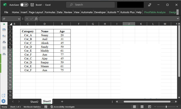
To understand the example of grouping age by using the pivot table. First consider the below given spreadsheet data −

Step 2

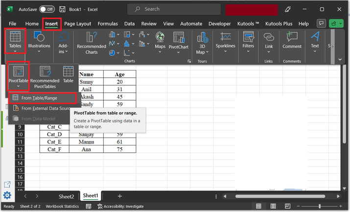
To create a pivot table, go to the “Insert” tab and then click on “Tables”. After that select the “PivotTable” option and choose the option “From Table/Range”.

Step 3

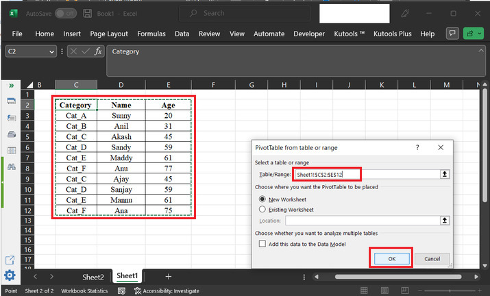
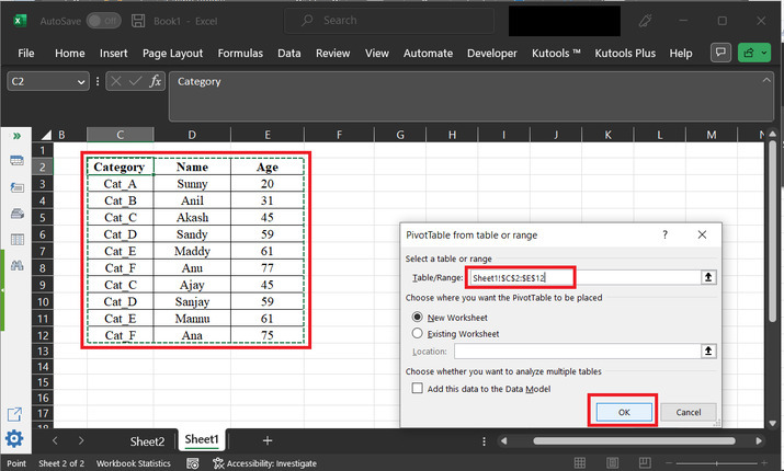
This will open the “PivotTable from table or range” dialog box. In the table/range section, select the complete data from the table, required user need to manipulate the data to produce required data.

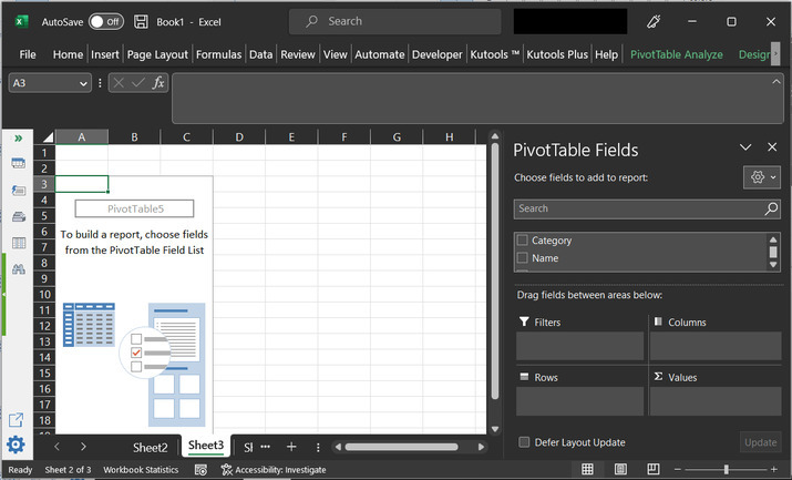
Step 4

This will display the below provided view. And, on the right-hand side. A “PivotTable Fields” section is displayed. In this section, user need to drag the fields between the provided fields. To obtain the data in the required format.

Step 5

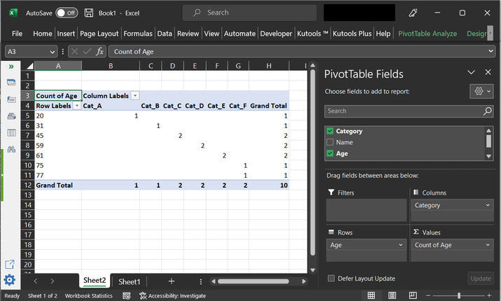
In the “PivotTable Field”. The user needs to tick the options “Category” and “Age”. After that drag the fields between the below given areas −

• In the columns areas drag the value “Category”.

• In the rows area drag the value “Age”

• In the “values” data, drag the values “Count of Age”.

This will modify the table and display a pivot table as shown left side. This pivot table will contain the row, and column labels. For proper understanding refer to the below provided data −

Step 6

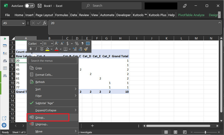
After that choose any row data, and right click on the row, to choose the option “Group…”. Consider the below depicted option −

Step 7

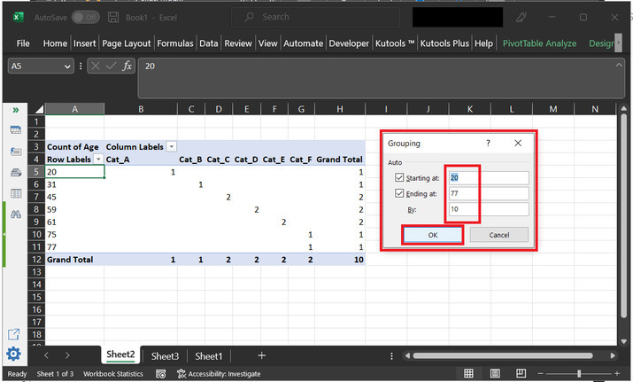
The above step will display a “Grouping” dialog box. This dialog box will contain labels for “Starting at” and “Ending at”. Tick both the options. This will make the input label editable. In the “Starting at” data enter the value as 20, (20 for this case only, as the provided data contains 20, as a starting age) and at the “Ending at” value type the last data value, for this case the last possible data value is 77. After that in the “By” label type the data range. For this example, the chosen value is 10. After that click on “OK”. Final snapshot of data is shown below −

Step 8

The final calculated data will contain the age as a range of data with the gap of 10 years. Consider the final output, as shown below −

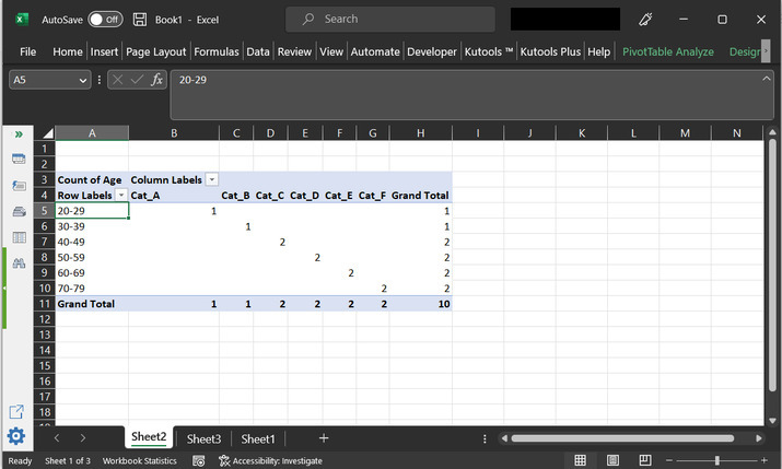
Conclusion

After properly following and learning all the above-provided steps, the user will be able to generate the pivot table and group the age data in the pivot table. The same method can also be used to group the other data available in Excel, according to the user's needs and requirements.