How to add image as background into chart in Excel?

In order to make the data more understandable, we need to include charts in the majority of the Excel files. In addition, we can either put a photo as the backdrop of the chart or fill the chart background with colour to make it more obvious.

This tutorial will provide you with an in-depth breakdown of how to put the aforementioned features into action, along with detailed instructions and images. If you follow all of the procedures, you will ultimately be able to fill up the chart backdrop with the appropriate colour or image.

Step 1

Fill in the necessary information for plot chat to provide a description of the added picture as the background.

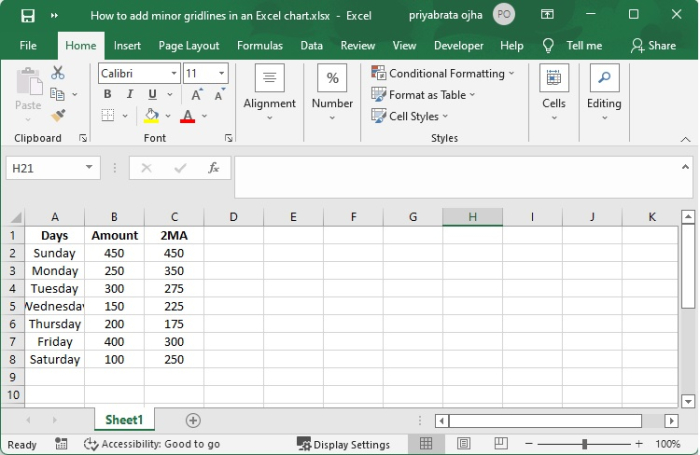
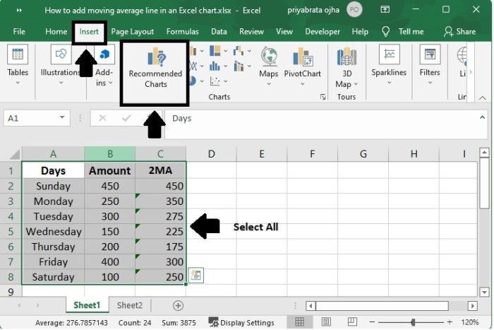
Step 2

Choose the data from the source, being sure to include the Average column (A1:C8).

Click Recommended Charts by going to the Insert tab, then clicking on the Charts group.

Step 3

Click the All Charts tab, then choose the Clustered Column − Line template, and then click the OK button.

If none of the standard combination charts meet your requirements, you may pick the Custom Combination type (the final template with the pen icon), and then choose the appropriate type for each of the data series.

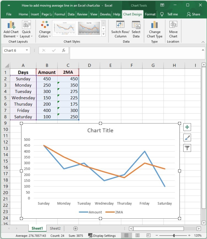
Step 4

The results of the line chart are as follows −

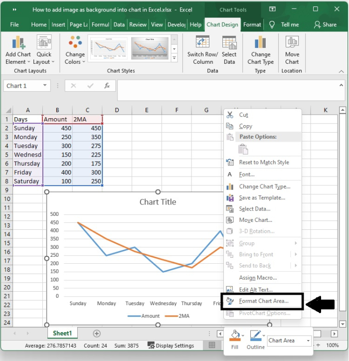
Step 5

You may load the chart management menu by clicking the right mouse button after selecting the whole chart by clicking on the margin. Choose the "Format Chart Area" option.

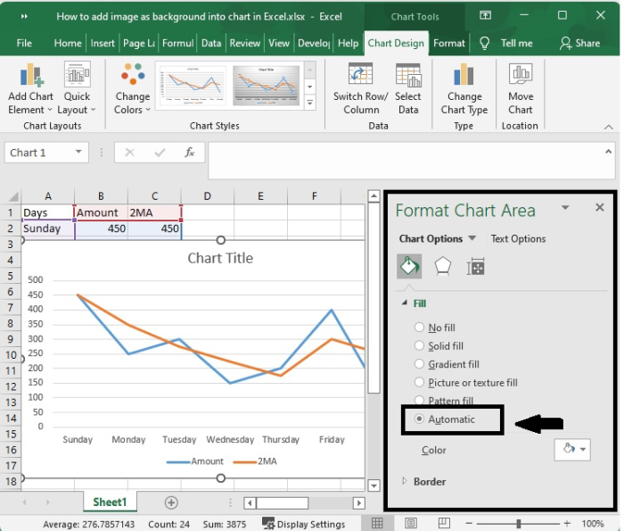
Step 6

Click the first icon labelled "Fill & Line" in the Chart Options section of the Format Chart Area. The option to use Automatic is selected by default.

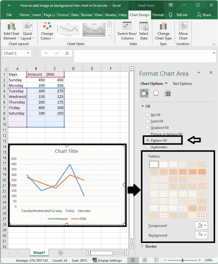
Step 7

Pattern fill − Check your chart when it comes to this. You are able to check to see whether the colour you picked is filled in the chart.

Step 8

Picture or texture fill − If you wish to add some texture to the backdrop of your chart, choose the texture option and choose one of the available options.

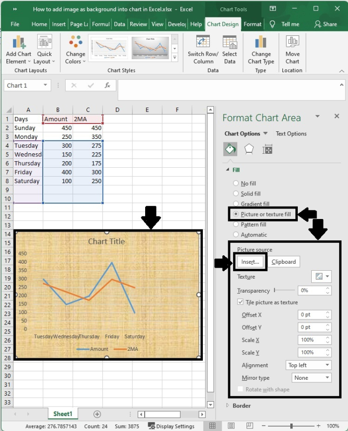
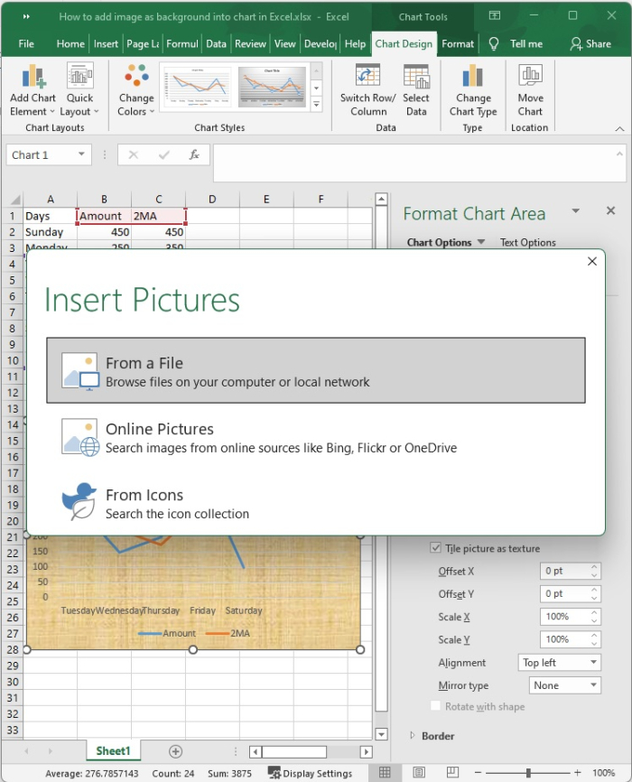
Step 9

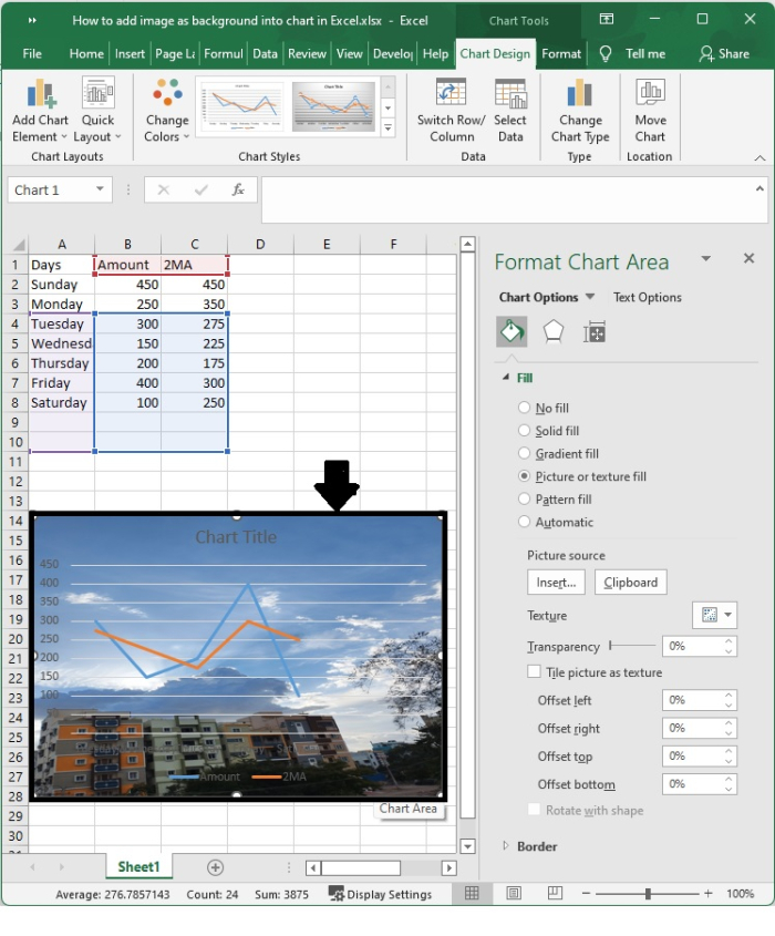
If you want to add an image to the chart background so that it is filled with some kind of background picture, then you should choose the insert option and choose one of the options that adds an image appropriately.

Step 10

The selected picture will serve as the background.

Step 11

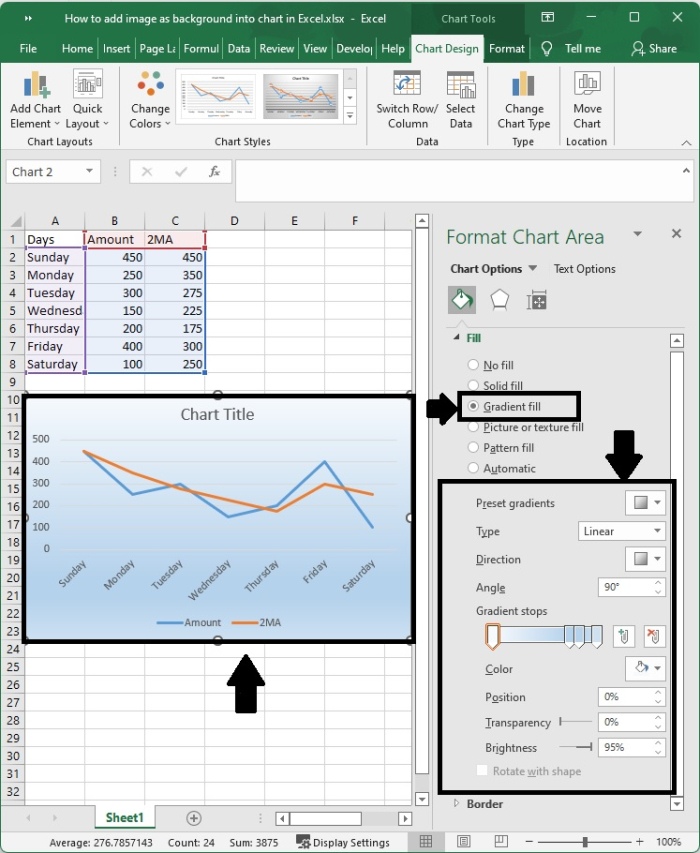
Gradient fill − Select Gradient fill in the Fill section and then use the options as shown in the following screenshot to set a gradient as the background of the chart.

Step 12

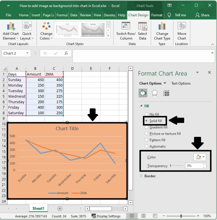
Solid fill − In the Fill settings section, select the "Solid fill" option, and then select a color from the Fill Color dropdown list to use as the background color.

Step 13

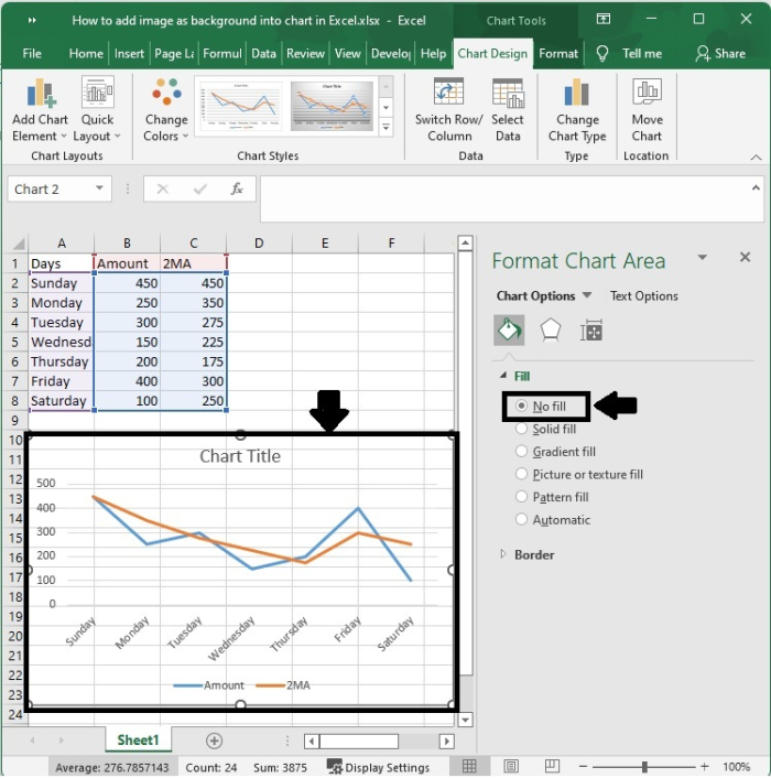
No fill − You may also modify Transparency per your requirement.

Conclusion

In this tutorial, we explained how you can use the different features of Excel to set the background of a chart on a worksheet.