Quick Guide

---

---

Introduction

The instruments, which are used to measure any quantity are known as measuring instruments. This tutorial covers mainly the electronic instruments, which are useful for measuring either electrical quantities or parameters.

Following are the most commonly used electronic instruments.

• Voltmeter
• Ammeter
• Ohmmeter
• Multimeter

Now, let us discuss about these instruments briefly.

Voltmeter

As the name suggests, voltmeter is a measuring instrument which measures the voltage across any two points of an electric circuit. There are two types of voltmeters: DC voltmeter, and AC voltmeter.

DC voltmeter measures the DC voltage across any two points of an electric circuit, whereas AC voltmeter measures the AC voltage across any two points of an electric circuit. An example of practical DC voltmeter is shown in below figure.

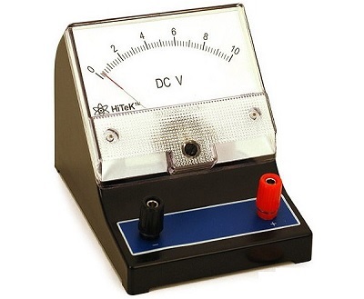
The DC voltmeter shown in above figure is a $(0-100)V$ DC voltmeter. Hence, it can be used to measure the DC voltages from zero volts to 10 volts.

Ammeter

As the name suggests, ammeter is a measuring instrument which measures the current flowing through any two points of an electric circuit. There are two types of ammeters: DC ammeter, and AC ammeter.

DC ammeter measures the DC current that flows through any two points of an electric circuit. Whereas, AC ammeter measures the AC current that flows through any two points of an electric circuit. An example of practical AC ammeter is shown in below figure −

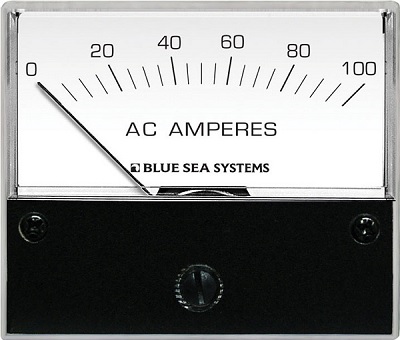
The AC ammeter shown in above figure is a $(0-100)A \:$ AC ammeter. Hence, it can be used to measure the AC currents from zero Amperes to 100 Amperes.

Ohmmeter

Ohmmeter is used to measure the value of resistance between any two points of an electric circuit. It can also be used for finding the value of an unknown resistor. There are two types of ohmmeters: series ohmmeter, and shunt ohmmeter.

In series type ohmmeter, the resistor whose value is unknown and to be measured should be connected in series with the ohmmeter. It is useful for measuring high values of resistances.

In shunt type ohmmeter, the resistor whose value is unknown and to be measured should be connected in parallel (shunt) with the ohmmeter. It is useful for measuring low values of resistances.

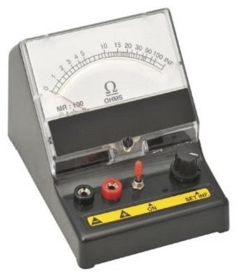
An example of practical shunt ohmmeter is shown in the above figure. The ohmmeter shown in above figure is a $(0-100)\Omega$ shunt ohmmeter. Hence, it can be used to measure the resistance values from zero ohms to 100 ohms.

Multimeter

Multimeter is an electronic instrument used to measure the quantities such as voltage, current & resistance one at a time. It can be used to measure DC & AC voltages, DC & AC currents and resistances of several ranges. A practical multimeter is shown in the following figure −

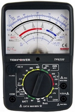
As shown in the figure, this multimeter can be used to measure various high resistances, low resistances, DC voltages, AC voltages, DC currents, & AC currents. Different scales and range of values for each of these quantities are marked in above figure.

The instruments which we considered in this chapter are of indicating type instruments, as the pointers of these instruments deflect and point to a particular value. We will discuss about these electronic measuring instruments in detail in later chapters.

Performance Characteristics

The characteristics of measurement instruments which are helpful to know the performance of instrument and help in measuring any quantity or parameter, are known as Performance Characteristics.

Types of Performance Characteristics

Performance characteristics of instruments can be classified into the following two types.

• Static Characteristics
• Dynamic Characteristics

Now, let us discuss about these two types of characteristics one by one.

Static Characteristics

The characteristics of quantities or parameters measuring instruments that do not vary with respect to time are called static characteristics. Sometimes, these quantities or parameters may vary slowly with respect to time. Following are the list of static characteristics.

• Accuracy
• Precision
• Sensitivity
• Resolution
• Static Error

Now, let us discuss about these static characteristics one by one.

Accuracy

The algebraic difference between the indicated value of an instrument, $A_{i}$ and the true value, $A_{t}$ is known as accuracy. Mathematically, it can be represented as −

$$Accuracy = A_{i}- A_{t}$$

The term, accuracy signifies how much the indicated value of an instrument, $A_{i}$ is closer to the true value, $A_{t}$.

Static Error

The difference between the true value, $A_{t}$ of the quantity that does not vary with respect to time and the indicated value of an instrument, $A_{i}$ is known as static error, $e_{s}$. Mathematically, it can be represented as −

$$e_{s}= A_{t}- A_{i}$$

The term, static error signifies the inaccuracy of the instrument. If the static error is represented in terms of percentage, then it is called percentage of static error. Mathematically, it can be represented as −

$$\% e_{s}=\frac{e_{s}}{A_{t}}\times 100$$

Substitute, the value of $e_{s}$ in the right hand side of above equation −

$$\% e_{s}=\frac{A_{t}- A_{i}}{A_{t}}\times 100$$

Where,

$\% e_{s}$ is the percentage of static error.

Precision

If an instrument indicates the same value repeatedly when it is used to measure the same quantity under same circumstances for any number of times, then we can say that the instrument has high precision.

Sensitivity

The ratio of change in output, $\Delta A_{out}$ of an instrument for a given change in the input, $\Delta A_{in}$ that is to be measured is called sensitivity, S. Mathematically it can be represented as −

$$S=\frac{\Delta A_{out}}{\Delta A_{in}}$$

The term sensitivity signifies the smallest change in the measurable input that is required for an instrument to respond.

• If the calibration curve is linear, then the sensitivity of the instrument will be a constant and it is equal to slope of the calibration curve.

• If the calibration curve is non-linear, then the sensitivity of the instrument will not be a constant and it will vary with respect to the input.

Resolution

If the output of an instrument will change only when there is a specific increment of the input, then that increment of the input is called Resolution. That means, the instrument is capable of measuring the input effectively, when there is a resolution of the input.

Dynamic Characteristics

The characteristics of the instruments, which are used to measure the quantities or parameters that vary very quickly with respect to time are called dynamic characteristics. Following are the list of dynamic characteristics.

• Speed of Response
• Dynamic Error
• Fidelity
• Lag

Now, let us discuss about these dynamic characteristics one by one.

Speed of Response

The speed at which the instrument responds whenever there is any change in the quantity to be measured is called speed of response. It indicates how fast the instrument is.

Lag

The amount of delay present in the response of an instrument whenever there is a change in the quantity to be measured is called measuring lag. It is also simply called lag.

Dynamic Error

The difference between the true value, $A_{t}$ of the quantity that varies with respect to time and the indicated value of an instrument, $A_{i}$ is known as dynamic error, $e_{d}$.

Fidelity

The degree to which an instrument indicates changes in the measured quantity without any dynamic error is known as Fidelity

Electronic Measuring Instruments - Errors

The errors, which occur during measurement are known as measurement errors. In this chapter, let us discuss about the types of measurement errors.

Types of Measurement Errors

We can classify the measurement errors into the following three types.

• Gross Errors
• Random Errors
• Systematic Errors

Now, let us discuss about these three types of measurement errors one by one.

Gross Errors

The errors, which occur due to the lack of experience of the observer while taking the measurement values are known as gross errors. The values of gross errors will vary from observer to observer. Sometimes, the gross errors may also occur due to improper selection of the instrument. We can minimize the gross errors by following these two steps.

• Choose the best suitable instrument, based on the range of values to be measured.
• Note down the readings carefully

Systematic Errors

If the instrument produces an error, which is of a constant uniform deviation during its operation is known as systematic error. The systematic errors occur due to the characteristics of the materials used in the instrument.

Types of Systematic Errors

The systematic errors can be classified into the following three types.

• Instrumental Errors − This type of errors occur due to shortcomings of instruments and loading effects.

• Environmental Errors − This type of errors occur due to the changes in environment such as change in temperature, pressure & etc.

• observational Errors − This type of errors occur due to observer while taking the meter readings. Parallax errors belong to this type of errors.

Random Errors

The errors, which occur due to unknown sources during measurement time are known as random errors. Hence, it is not possible to eliminate or minimize these errors. But, if we want to get the more accurate measurement values without any random error, then it is possible by following these two steps.

• Step1 − Take more number of readings by different observers.

• Step2 − Do statistical analysis on the readings obtained in Step1.

Following are the parameters that are used in statistical analysis.

• Mean
• Median
• Variance
• Deviation
• Standard Deviation

Now, let us discuss about these statistical parameters.

Mean

Let $x_{1},x_{2},x_{3},....,x_{N}$ are the $N$ readings of a particular measurement. The mean or average value of these readings can be calculated by using the following formula.

$$m = \frac{x_{1}+x_{2}+x_{3}+....+x_{N}}{N}$$

Where, $m$ is the mean or average value.

If the number of readings of a particular measurement are more, then the mean or average value will be approximately equal to true value

Median

If the number of readings of a particular measurement are more, then it is difficult to calculate the mean or average value. Here, calculate the median value and it will be approximately equal to mean value.

For calculating median value, first we have to arrange the readings of a particular measurement in an ascending order. We can calculate the median value by using the following formula, when the number of readings is an odd number.

$$M=x_{\left ( \frac{N+1}{2} \right )}$$

We can calculate the median value by using the following formula, when the number of readings is an even number.

$$M=\frac{x_{\left ( N/2 \right )}+x_\left ( \left [ N/2 \right ]+1 \right )}{2}$$

Deviation from Mean

The difference between the reading of a particular measurement and the mean value is known as deviation from mean. In short, it is called deviation. Mathematically, it can be represented as

$$d_{i}=x_{i}-m$$

Where,

$d_{i}$ is the deviation of $i^{th}$ reading from mean.

$x_{i}$ is the value of $i^{th}$ reading.

$m$ is the mean or average value.

Standard Deviation

The root mean square of deviation is called standard deviation. Mathematically, it can be represented as

$$\sigma =\sqrt{\frac{{d_{1}}^{2}+{d_{2}}^{2}+{d_{3}}^{2}+....+{d_{N}}^{2}}{N}}$$

The above formula is valid if the number of readings, N is greater than or equal to 20. We can use the following formula for standard deviation, when the number of readings, N is less than 20.

$$\sigma =\sqrt{\frac{{d_{1}}^{2}+{d_{2}}^{2}+{d_{3}}^{2}+....+{d_{N}}^{2}}{N-1}}$$

Where,

$\sigma$ is the standard deviation

$d_{1}, d_{2}, d_{3}, …, d_{N}$ are the deviations of first, second, third, …, $N^{th}$readings from mean respectively.

Note − If the value of standard deviation is small, then there will be more accuracy in the reading values of measurement.

Variance

The square of standard deviation is called variance. Mathematically, it can be represented as

$$V=\sigma^{2}$$

Where,

$V$ is the variance

$\sigma$ is the standard deviation

The mean square of deviation is also called variance. Mathematically, it can be represented as

$$V=\frac{{d_{1}}^{2}+{d_{2}}^{2}+{d_{3}}^{2}+....+{d_{N}}^{2}}{N}$$

The above formula is valid if the number of readings, N is greater than or equal to 20. We can use the following formula for variance when the number of readings, N is less than 20.

$$V=\frac{{d_{1}}^{2}+{d_{2}}^{2}+{d_{3}}^{2}+....+{d_{N}}^{2}}{N-1}$$

Where,

$V$ is the variance

$d_{1}, d_{2}, d_{3}, …, d_{N}$ are the deviations of first, second, third, …, $N^{th}$ readings from mean respectively.

So, with the help of statistical parameters, we can analyze the readings of a particular measurement. In this way, we will get more accurate measurement values.

Electronic Measuring Instruments

The instruments used to measure any quantity are known as measuring instruments. If the instruments can measure the basic electrical quantities, such as voltage and current are known as basic measuring instruments.

Types of Basic Measuring Instruments

We can classify the basic measuring instruments into the following two types.

• Voltmeters
• Ammeters

Let us discuss about these two basic measuring instruments briefly.

Voltmeters

As the name suggests, voltmeter is a measuring instrument which measures the voltage across any two points of an electric circuit. The units of voltage are volt and the measuring instrument is meter. Hence, the word “voltmeter” is obtained by combining the two words “volt” and “meter”.

We can classify the voltmeters into the following two types based on the type of voltage that it can measure.

• DC Voltmeters
• AC Voltmeters

DC Voltmeter

As the name suggests, DC voltmeter measures the DC voltage across any two points of an electric circuit. A practical DC voltmeter is shown in below figure.

The DC voltmeter shown in the figure is a $(0-10)V$ DC voltmeter. Hence, it can be used to measure the DC voltages from zero volts to 10 volts

AC Voltmeter

As the name suggests, AC voltmeter measures the AC voltage across any two points of an electric circuit. A practical AC voltmeter is shown in below figure.

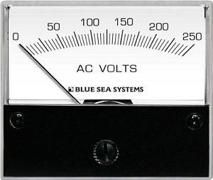
The AC voltmeter shown in above figure is a $(0-250)V$ AC voltmeter. Hence, it can be used to measure the AC voltages from zero volts to 250 volts

Ammeters

As the name suggests, ammeter is a measuring instrument which measures the current flowing through any two points of an electric circuit. The unit of current is ampere and the measuring instrument is meter. The word “ammeter” is obtained by combining “am” of ampere with “meter”.

We can classify the ammeters into the following two types based on the type of current that it can measure.

• DC Ammeters
• AC Ammeters

DC Ammeter

As the name suggests, DC ammeter measures the DC current that flows through any two points of an electric circuit. A practical DC ammeter is shown in figure.

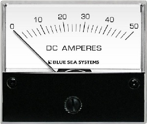
The DC ammeter shown in above figure is a $(0-50)A$ DC ammeter. Hence, it can be used to measure the DC currents from zero Amperes to 50 Amperes

AC Ammeter

As the name suggests, AC ammeter measures the AC current that flows through any two points of an electric circuit. A practical AC ammeter is shown in below figure.

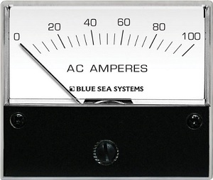
The AC ammeter shown in above figure is a $(0-100)A$ AC ammeter. Hence, it can be used to measure the AC currents from zero Amperes to 100 Amperes.

We will discuss about various voltmeters and ammeters in detail in the following few chapters

DC Voltmeters

DC voltmeter is a measuring instrument, which is used to measure the DC voltage across any two points of electric circuit. If we place a resistor in series with the Permanent Magnet Moving Coil (PMMC) galvanometer, then the entire combination together acts as DC voltmeter.

The series resistance, which is used in DC voltmeter is also called series multiplier resistance or simply, multiplier. It basically limits the amount of current that flows through galvanometer in order to prevent the meter current from exceeding the full scale deflection value. The circuit diagram of DC voltmeter is shown in below figure.

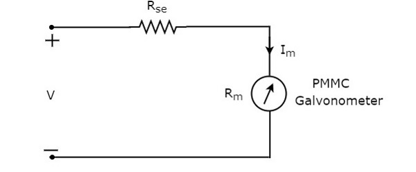
We have to place this DC voltmeter across the two points of an electric circuit, where the DC voltage is to be measured.

Apply KVL around the loop of above circuit.

$V-I_{m}R_{se}-I_{m}R_{m}=0$ (Equation 1)

$$\Rightarrow V-I_{m}R_{m}=I_{m}R_{se}$$

$$\Rightarrow R_{se}=\frac{V-I_{m}R_{m}}{I_{m}}$$

$\Rightarrow R_{se}=\frac{V}{I_{m}}-R_{m}$ (Equation 2)

Where,

$R_{se}$ is the series multiplier resistance

$V$ is the full range DC voltage that is to be measured

$I_{m}$ is the full scale deflection current

$R_{m}$ is the internal resistance of galvanometer

The ratio of full range DC voltage that is to be measured, $V$ and the DC voltage drop across the galvanometer, $V_{m}$ is known as multiplying factor, m. Mathematically, it can be represented as

$m=\frac{V}{V_{m}}$ (Equation 3)

From Equation 1, we will get the following equation for full range DC voltage that is to be measured, $V$.

$V=I_{m}R_{se}+I_{m}R_{m}$ (Equation 4)

The DC voltage drop across the galvanometer, $V_{m}$ is the product of full scale deflection current, $I_{m}$ and internal resistance of galvanometer, $R_{m}$. Mathematically, it can be written as

$V_{m}=I_{m}R_{m}$ (Equation 5)

Substitute, Equation 4 and Equation 5 in Equation 3.

$$m=\frac{I_{m}R_{se}+I_{m}R_{m}}{I_{m}R_{m}}$$

$\Rightarrow m=\frac{R_{se}}{R_{m}}+1$

$\Rightarrow m-1=\frac{R_{se}}{R_{m}}$

$R_{se}=R_{m}\left (m-1 \right )$(Equation 6)

We can find the value of series multiplier resistance by using either Equation 2 or Equation 6 based on the available data.

Multi Range DC Voltmeter

In previous section, we had discussed DC voltmeter, which is obtained by placing a multiplier resistor in series with the PMMC galvanometer. This DC voltmeter can be used to measure a particular range of DC voltages.

If we want to use the DC voltmeter for measuring the DC voltages of multiple ranges, then we have to use multiple parallel multiplier resistors instead of single multiplier resistor and this entire combination of resistors is in series with the PMMC galvanometer. The circuit diagram of multi range DC voltmeter is shown in below figure.

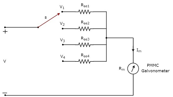
We have to place this multi range DC voltmeter across the two points of an electric circuit, where the DC voltage of required range is to be measured. We can choose the desired range of voltages by connecting the switch s to the respective multiplier resistor.

Let, $m_{1},m_{2}, m_{2} $ and $m_{4}$ are the multiplying factors of DC voltmeter when we consider the full range DC voltages to be measured as, $V_{1} , V_{2}, V_{3}$ and $V_{4}$ respectively. Following are the formulae corresponding to each multiplying factor.

$$m_{1}=\frac{V_{1}}{V_{m}}$$

$$m_{2}=\frac{V_{2}}{V_{m}}$$

$$m_{3}=\frac{V_{3}}{V_{m}}$$

$$m_{4}=\frac{V_{4}}{V_{m}}$$

In above circuit, there are four series multiplier resistors, $R_{se1}, R_{se2}, R_{se3}$ and $R_{se4}$. Following are the formulae corresponding to these four resistors.

$$R_{se1}=R_{m}\left (m_{1}-1 \right )$$

$$R_{se2}=R_{m}\left (m_{2}-1 \right )$$

$$R_{se3}=R_{m}\left (m_{3}-1 \right )$$

$$R_{se4}=R_{m}\left (m_{4}-1 \right )$$

So, we can find the resistance values of each series multiplier resistor by using above formulae.

AC Voltmeters

The instrument, which is used to measure the AC voltage across any two points of electric circuit is called AC voltmeter. If the AC voltmeter consists of rectifier, then it is said to be rectifier based AC voltmeter.

The DC voltmeter measures only DC voltages. If we want to use it for measuring AC voltages, then we have to follow these two steps.

• Step1 − Convert the AC voltage signal into a DC voltage signal by using a rectifier.

• Step2 − Measure the DC or average value of the rectifier’s output signal.

We get Rectifier based AC voltmeter, just by including the rectifier circuit to the basic DC voltmeter. This chapter deals about rectifier based AC voltmeters.

Types of Rectifier based AC Voltmeters

Following are the two types of rectifier based AC voltmeters.

• AC voltmeter using Half Wave Rectifier
• AC voltmeter using Full Wave Rectifier

Now, let us discuss about these two AC voltmeters one by one.

AC Voltmeter using Half Wave Rectifier

If a Half wave rectifier is connected ahead of DC voltmeter, then that entire combination together is called AC voltmeter using Half wave rectifier. The block diagram of AC voltmeter using Half wave rectifier is shown in below figure.

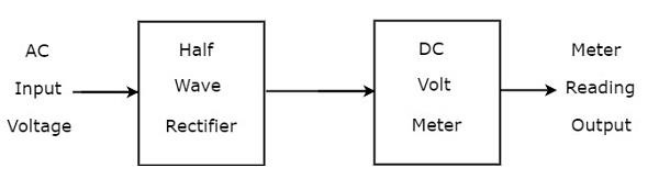
The above block diagram consists of two blocks: half wave rectifier and DC voltmeter. We will get the corresponding circuit diagram, just by replacing each block with the respective component(s) in above block diagram. So, the circuit diagram of AC voltmeter using Half wave rectifier will look like as shown in below figure.

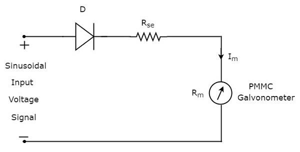
The rms value of sinusoidal (AC) input voltage signal is

$$V_{rms}=\frac{V_{m}}{\sqrt{2}}$$

$$\Rightarrow V_{m}=\sqrt{2} V_{rms}$$

$$\Rightarrow V_{m}=1.414 V_{rms}$$

Where,

$V_{m}$ is the maximum value of sinusoidal (AC) input voltage signal.

The DC or average value of the Half wave rectifier’s output signal is

$$V_{dc}=\frac{V_{m}}{\pi}$$

Substitute, the value of $V_{m}$ in above equation.

$$V_{dc}= \frac{1.414 V_{rms}}{\pi}$$

$$V_{dc}= 0.45 V_{rms}$$

Therefore, the AC voltmeter produces an output voltage, which is equal to 0.45 times the rms value of the sinusoidal (AC) input voltage signal

AC Voltmeter using Full Wave Rectifier

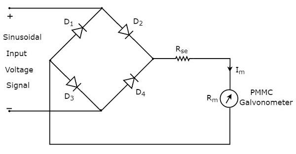
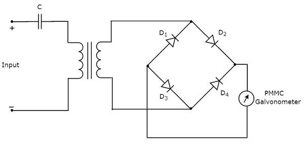
If a Full wave rectifier is connected ahead of DC voltmeter, then that entire combination together is called AC voltmeter using Full wave rectifier. The block diagram of AC voltmeter using Full wave rectifier is shown in below figure

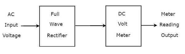
The above block diagram consists of two blocks: full wave rectifier and DC voltmeter. We will get the corresponding circuit diagram just by replacing each block with the respective component(s) in above block diagram.

So, the circuit diagram of AC voltmeter using Full wave rectifier will look like as shown in below figure.

The rms value of sinusoidal (AC) input voltage signal is

$$V_{rms}=\frac{V_{m}}{\sqrt{2}}$$

$$\Rightarrow V_{m}=\sqrt{2} \:V_{rms}$$

$$\Rightarrow V_{m}= 1.414 V_{rms}$$

Where,

$V_{m}$ is the maximum value of sinusoidal (AC) input voltage signal.

The DC or average value of the Full wave rectifier’s output signal is

$$V_{dc}=\frac{2V_{m}}{\pi}$$

Substitute, the value of $V_{m}$ in above equation

$$V_{dc}=\frac{2\times 1.414 \:V_{rms}}{\pi}$$

$$V_{dc}=0.9 \:V_{rms}$$

Therefore, the AC voltmeter produces an output voltage, which is equal to 0.9 times the rms value of the sinusoidal (AC) input voltage signal.

Other AC Voltmeters

In previous chapter, we discussed about rectifier based AC voltmeters. This chapter covers the following two types of AC voltmeters.

• Peak responding AC voltmeter
• True RMS responding AC voltmeter

Now, let us discuss about these two types of AC voltmeters one by one.

Peak Responding AC Voltmeter

As the name suggests, the peak responding AC voltmeter responds to peak values of AC voltage signal. That means, this voltmeter measures peak values of AC voltages. The circuit diagram of peak responding AC voltmeter is shown below −

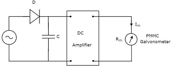
The above circuit consists of a diode, capacitor, DC amplifier and PMMC galvanometer. The diode present in the above circuit is used for rectification purpose. So, the diode converts AC voltage signal into a DC voltage signal. The capacitor charges to the peak value of this DC voltage signal.

During positive half cycle of AC voltage signal, the diode conducts and the capacitor charges to the peak value of AC voltage signal. When the value of AC voltage signal is less than this value, the diode will be reverse biased.

Thus, the capacitor will discharge through resistor of DC amplifier till the next positive half cycle of AC voltage signal. When the value of AC voltage signal is greater than the capacitor voltage, the diode conducts and the process will be repeated.

We should select the component values in such a way that the capacitor charges fast and discharges slowly. As a result, the meter always responds to this capacitor voltage, i.e. the peak value of AC voltage.

True RMS Responding AC Voltmeter

As the name suggests, the true RMS responding AC voltmeter responds to the true RMS values of AC voltage signal. This voltmeter measures RMS values of AC voltages. The circuit diagram of true RMS responding AC voltmeter is shown in below figure.

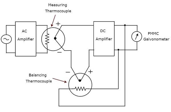
The above circuit consists of an AC amplifier, two thermocouples, DC amplifier and PMMC galvanometer. AC amplifier amplifies the AC voltage signal. Two thermocouples that are used in above circuit are a measuring thermocouple and a balancing thermocouple. Measuring thermocouple produces an output voltage, which is proportional to RMS value of the AC voltage signal.

Any thermocouple converts a square of input quantity into a normal quantity. This means there exists a non-linear relationship between the output and input of a thermocouple. The effect of non-linear behavior of a thermocouple can be neglected by using another thermocouple in the feedback circuit. The thermocouple that is used for this purpose in above circuit is known as balancing thermocouple.

The two thermocouples, namely measuring thermocouple and balancing thermocouple together form a bride at the input of DC amplifier. As a result, the meter always responds to the true RMS value of AC voltage signal.

DC Ammeters

Current is the rate of flow of electric charge. If this electric charge flows only in one direction, then the resultant current is called Direct Current (DC). The instrument, which is used to measure the Direct Current called DC ammeter.

If we place a resistor in parallel with the Permanent Magnet Moving Coil (PMMC) galvanometer, then the entire combination acts as DC ammeter. The parallel resistance, which is used in DC ammeter is also called shunt resistance or simply, shunt. The value of this resistance should be considered small in order to measure the DC current of large value.

The circuit diagram of DC ammeter is shown in below figure.

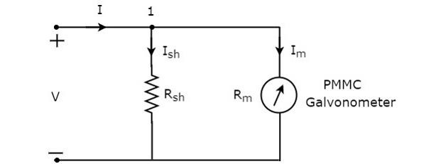
We have to place this DC ammeter in series with the branch of an electric circuit, where the DC current is to be measured. The voltage across the elements, which are connected in parallel is same. So, the voltage across shunt resistor, $R_{sh}$ and the voltage across galvanometer resistance, $R_{m}$ is same, since those two elements are connected in parallel in above circuit. Mathematically, it can be written as

$$I_{sh}R_{sh}=I_{m}R_{m}$$

$\Rightarrow R_{sh}=\frac{I_{m}R_{m}}{I_{sh}}$ (Equation 1)

The KCL equation at node 1 is

$$-I+I_{sh}+I_{m}=0$$

$$\Rightarrow I_{sh}=I-I_{m}$$

Substitute the value of $I_{sh}$ in Equation 1.

$R_{sh}=\frac{I_{m}R_{m}}{I-I_{m}}$(Equation 2)

Take, $I_{m}$ as common in the denominator term, which is present in the right hand side of Equation 2

$$R_{sh}=\frac{I_{m}R_{m}}{I_{m}(\frac{1}{I_{m}}-1)}$$

$\Rightarrow R_{sh}=\frac{R_{m}}{\frac{I}{I_{m}}-1}$(Equation 3)

Where,

$R_{sh}$ is the shunt resistance

$R_{m}$ is the internal resistance of galvanometer

$I$ is the total Direct Current that is to be measured

$I_{m}$ is the full scale deflection current

The ratio of total Direct Current that is to be measured, $I$ and the full scale deflection current of the galvanometer, $I_{m}$ is known as multiplying factor, m. Mathematically, it can be represented as

$m=\frac{I}{I_{m}}$(Equation 4)

$R_{sh}=\frac{R_{m}}{m-1}$(Equation 5)

We can find the value of shunt resistance by using either Equation 2 or Equation 5 based on the available data.

Multi Range DC Ammeter

In previous section, we discussed about DC ammeter which is obtained by placing a resistor in parallel with the PMMC galvanometer. This DC ammeter can be used to measure a particular range of Direct Currents.

If we want to use the DC ammeter for measuring the Direct Currents of multiple ranges, then we have to use multiple parallel resistors instead of single resistor and this entire combination of resistors is in parallel to the PMMC galvanometer. The circuit diagram of multi range DC ammeter is shown in below figure.

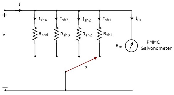
Place this multi range DC ammeter in series with the branch of an electric circuit, where the Direct Current of required range is to be measured. The desired range of currents is chosen by connecting the switch, s to the respective shunt resistor.

Let, $m_{1}, m_{2}, m_{3}$ and $m_{4}$ are the multiplying factors of DC ammeter when we consider the total Direct Currents to be measured as, $I_{1}, I_{2}, I_{3}$ and $I_{4}$ respectively. Following are the formulae corresponding to each multiplying factor.

$$m_{1}=\frac{I_{1}}{I_{m}}$$

$$m_{2}=\frac{I_{2}}{I_{m}}$$

$$m_{3}=\frac{I_{3}}{I_{m}}$$

$$m_{4}=\frac{I_{4}}{I_{m}}$$

In above circuit, there are four shunt resistors, $R_{sh1}, R_{sh2}, R_{sh2}$ and $R_{sh4}$. Following are the formulae corresponding to these four resistors.

$$R_{sh1}=\frac{R_{m}}{m_{1}-1}$$

$$R_{sh2}=\frac{R_{m}}{m_{2}-1}$$

$$R_{sh3}=\frac{R_{m}}{m_{3}-1}$$

$$R_{sh4}=\frac{R_{m}}{m_{4}-1}$$

The above formulae will help us find the resistance values of each shunt resistor.

AC Ammeter

Current is the rate of flow of electric charge. If the direction of this electric charge changes regularly, then the resultant current is called Alternating Current (AC).

The instrument, which is used to measure the Alternating Current that flows through any branch of electric circuit is called AC ammeter.

Example − Thermocouple type AC ammeter.

Now, let us discuss about Thermocouple type AC ammeter.

Thermocouple Type AC Ammeter

If a Thermocouple is connected ahead of PMMC galvanometer, then that entire combination is called thermocouple type AC ammeter. The block diagram of thermocouple type AC ammeter is shown in below figure.

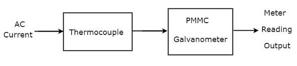
The above block diagram consists of mainly two blocks: a thermocouple, and a PMMC galvanometer. We will get the corresponding circuit diagram, just by replacing each block with the respective component(s) in above block diagram. So, the circuit diagram of thermocouple type AC ammeter will look like as shown in below figure.

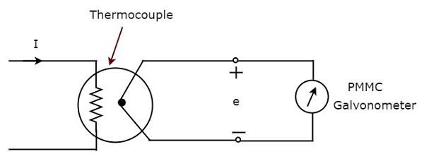
Thermocouple generates an EMF, $e$, whenever the Alternating Current, I flows through heater element. This EMF, $e$ is directly proportional to the rms value of the current, I that is flowing through heater element. So, we have to calibrate the scale of PMMC instrument to read rms values of current.

So, with this chapter we have completed all basic measuring instruments such as DC voltmeters, AC voltmeters, DC ammeters and AC ammeters. In next chapter, let us discuss about the meters or measuring instruments, which measure resistance value.

OHMMeters

The instrument, which is used to measure the value of resistance between any two points in an electric circuit is called ohmmeter. It can also be used to find the value of an unknown resistor. The units of resistance are ohm and the measuring instrument is meter. So, the word “ohmmeter” is obtained by combining the words “ohm” and “meter”.

Types of Ohmmeters

Following are the two types of ohmmeters.

• Series Ohmmeter
• Shunt Ohmmeter

Now, let us discuss about these two types of ohmmeters one by one.

Series Ohmmeter

If the resistor’s value is unknown and has to be measured by placing it in series with the ohmmeter, then that ohmmeter is called series ohmmeter. The circuit diagram of series ohmmeter is shown in below figure.

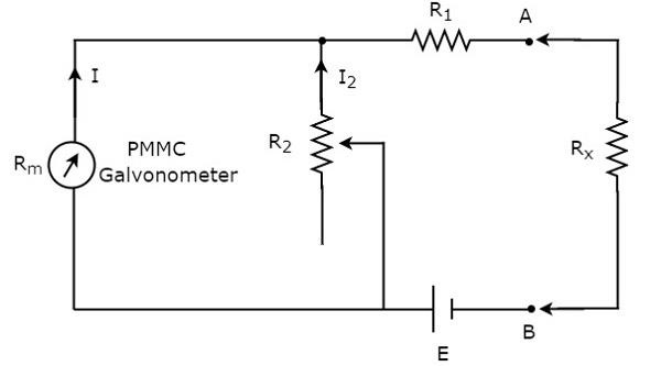
The part of the circuit, which is left side of the terminals A & B is series ohmmeter. So, we can measure the value of unknown resistance by placing it to the right side of terminals A & B. Now, let us discuss about the calibration scale of series ohmmeter.

• If $R_{x}= 0 \:\Omega$, then the terminals A & B will be short circuited with each other. So, the meter current gets divided between the resistors, $R_{1}$ and $R_{2}$. Now, vary the value of resistor, $R_{2}$ in such a way that the entire meter current flows through the resistor, $R_{1}$ only. In this case, the meter shows full scale deflection current. Hence, this full scale deflection current of the meter can be represented as $0 \:\Omega$.

• If $R_{x}= \infty \:\Omega$, then the terminals A & B will be open circuited with each other. So, no current flows through resistor, $R_{1}$. In this case, the meter shows null deflection current. Hence, this null deflection of the meter can be represented as $\infty \Omega$.

• In this way, by considering different values of $R_{x}$, the meter shows different deflections. So, accordingly we can represent those deflections with the corresponding resistance value.

The series ohmmeter consists of a calibration scale. It has the indications of 0 $\Omega$ and $\infty \:\Omega$ at the end points of right hand and left hand of the scale respectively. Series ohmmeter is useful for measuring high values of resistances.

Shunt Ohmmeter

If the resistor’s value is unknown and to be measured by placing it in parallel (shunt) with the ohmmeter, then that ohmmeter is called shunt ohmmeter. The circuit diagram of shunt ohmmeter is shown in below figure.

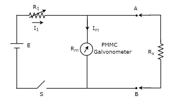
The part of the circuit, which is left side of the terminals A & B is shunt ohmmeter. So, we can measure the value of unknown resistance by placing it to the right side of terminals A & B.

Now, let us discuss about the calibration scale of shunt ohmmeter. Close the switch, S of above circuit while it is in use.

• If $R_{x}=0 \:\Omega$, then the terminals A & B will be short circuited with each other. Due to this, the entire current, $I_{1}$ flows through the terminals A & B. In this case, no current flows through PMMC galvanometer. Hence, the null deflection of the PMMC galvanometer can be represented as $0 \:\Omega$.

• If $R_{x}=\infty \:\Omega$, then the terminals A & B will be open circuited with each other. So, no current flows through the terminals A & B. In this case, the entire current, $I_{1}$ flows through PMMC galvanometer. If required vary (adjust) the value of resistor, $R_{1}$ until the PMMC galvanometer shows full scale deflection current. Hence, this full scale deflection current of the PMMC galvanometer can be represented as $\infty \:\Omega$

• In this way, by considering different values of $R_{x}$, the meter shows different deflections. So, accordingly we can represent those deflections with the corresponding resistance values.

The shunt ohmmeter consists of a calibration scale. It has the indications of $0 \:\Omega$ and $\infty \:\Omega$ at the end points of left hand and right hand of the scale respectively.

Shunt ohmmeter is useful for measuring low values of resistances. So, we can use either series ohmmeter or shunt ohmmeter based on the values of resistances that are to be measured i.e., high or low.

MultiMeter

In previous chapters, we discussed about voltmeters, ammeters and ohmmeters. These measuring instruments are used to measure voltage, current and resistance respectively. That means, we have separate measuring instruments for measuring voltage, current and resistance.

Suppose, if a single measuring instrument can be used to measure the quantities such as voltage, current & resistance one at a time, then it is said to be multimeter. It has got the name multimeter, since it can measure multiple electrical quantities one at a time.

Measurements by using Multimeter

Multimeter is an instrument used to measure DC & AC voltages, DC & AC currents and resistances of several ranges. It is also called Electronic Multimeter or Voltage Ohm Meter (VOM).

DC voltage Measurement

The part of the circuit diagram of Multimeter, which can be used to measure DC voltage is shown in below figure.

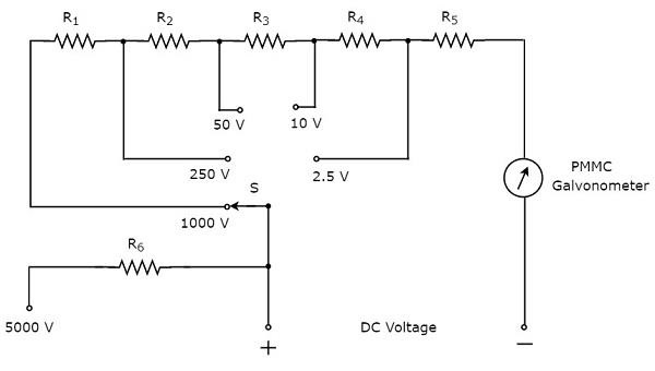
The above circuit looks like a multi range DC voltmeter. The combination of a resistor in series with PMMC galvanometer is a DC voltmeter. So, it can be used to measure DC voltages up to certain value.

We can increase the range of DC voltages that can be measured with the same DC voltmeter by increasing the resistance value. the equivalent resistance value increases, when we connect the resistors are in series.

In above circuit, we can measure the DC voltages up to 2.5V by using the combination of resistor, $R_{5}$ in series with PMMC galvanometer. By connecting a resistor, $R_{4}$ in series with the previous circuit, we can measure the DC voltages up to 10V. In this way, we can increase the range of DC voltages, simply by connecting a resistor in series with the previous (earlier) circuit.

We can measure the DC voltage across any two points of an electric circuit, by connecting the switch, S to the desired voltage range.

DC Current Measurement

The part of the circuit diagram of Multimeter, which can be used to measure DC current is shown in below figure.

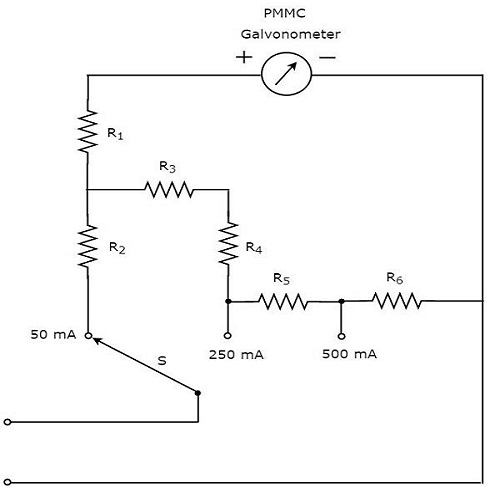
The above circuit looks like a multi range DC ammeter. the combination of a resistor in parallel with PMMC galvanometer is a DC ammeter. So, it can be used to measure DC currents up to certain value.

We can get different ranges of DC currents measured with the same DC ammeter by placing the resistors in parallel with previous resistor. In above circuit, the resistor, $R_{1}$ is connected in series with the PMMC galvanometer in order to prevent the meter gets damaged due to large current.

We can measure the DC current that is flowing through any two points of an electric circuit, by connecting the switch, S to the desired current range

AC voltage Measurement

The part of the circuit diagram of Multimeter, which can be used to measure AC voltage is shown in below figure.

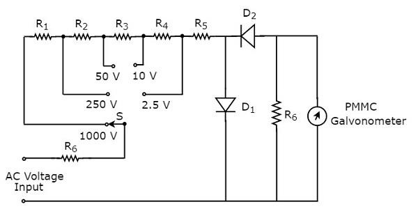
The above circuit looks like a multi range AC voltmeter. We know that, we will get AC voltmeter just by placing rectifier in series (cascade) with DC voltmeter. The above circuit was created just by placing the diodes combination and resistor, $R_{6}$ in between resistor, $R_{5}$ and PMMC galvanometer.

We can measure the AC voltage across any two points of an electric circuit, by connecting the switch, S to the desired voltage range.

Resistance Measurement

The part of the circuit diagram of Multimeter, which can be used to measure resistance is shown in below figure.

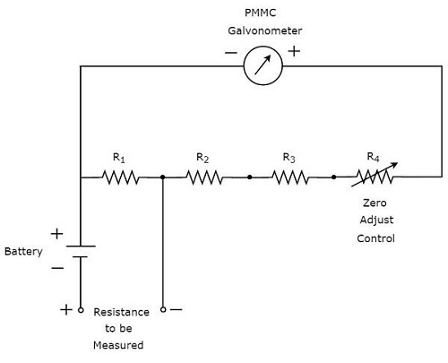
We have to do the following two tasks before taking any measurement.

• Short circuit the instrument
• Vary the zero adjust control until the meter shows full scale current. That means, meter indicates zero resistance value.

Now, the above circuit behaves as shunt ohmmeter and has the scale multiplication of 1, i.e. 10⁰. We can also consider higher order powers of 10 as the scale multiplications for measuring high resistances.

Signal Generators

Signal generator is an electronic equipment that provides standard test signals like sine wave, square wave, triangular wave and etc. It is also called an oscillator, since it produces periodic signals.

The signal generator, which produces the periodic signal having a frequency of Audio Frequency (AF) range is called AF signal generator. the range of audio frequencies is 20Hz to 20KHz.

AF Sine and Square Wave Generator

The AF signal generator, which generates either sine wave or square wave in the range of audio frequencies based on the requirement is called AF Sine and Square wave generator. Its block diagramis shown in below figure.

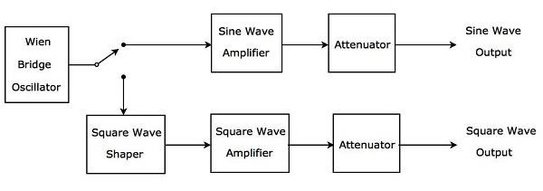
The above block diagram consists of mainly two paths. Those are upper path and lower path. Upper path is used to produce AF sine wave and the lower path is used to produce AF square wave.

Wien bridge oscillator will produce a sine wave in the range of audio frequencies. Based on the requirement, we can connect the output of Wien bridge oscillator to either upper path or lower path by a switch.

The upper path consists of the blocks like sine wave amplifier and attenuator. If the switch is used to connect the output of Wien bridge oscillator to upper path, it will produce a desired AF sine wave at the output of upper path.

The lower path consists of the following blocks: square wave shaper, square wave amplifier, and attenuator. The square wave shaper converts the sine wave into a square wave. If the switch is used to connect the output of Wien bridge oscillator to lower path, then it will produce a desired AF square wave at the output of lower path. In this way, the block diagram that we considered can be used to produce either AF sine wave or AF square wave based on the requirement.

Function Generator

Function generator is a signal generator, which generates three or more periodic waves. Consider the following block diagram of a Function generator, which will produce periodic waves like triangular wave, square wave and sine wave.

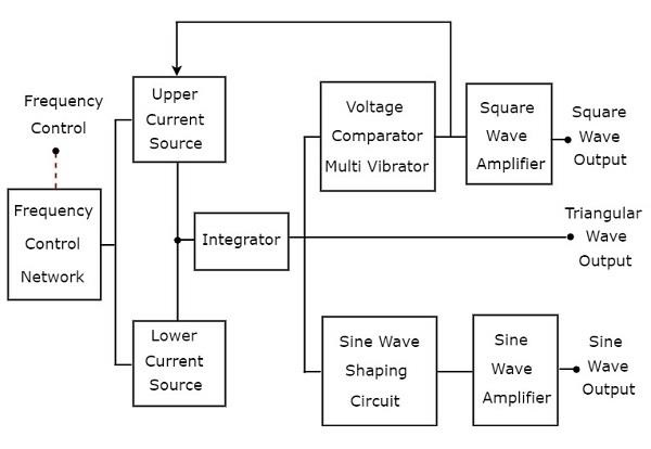
There are two current sources, namely upper current source and lower current source in above block diagram. These two current sources are regulated by the frequency-controlled voltage.

Triangular Wave

Integrator present in the above block diagram, gets constant current alternately from upper and lower current sources for equal amount of time repeatedly. So, the integrator will produce two types of output for the same time repeatedly −

• The output voltage of an integrator increases linearly with respect to time for the period during which integrator gets current from upper current source.

• The output voltage of an integrator decreases linearly with respect to time for the period during which integrator gets current from lower current source.

In this way, the integrator present in above block diagram will produce a triangular wave.

Square Wave & Sine Wave

The output of integrator, i.e. the triangular wave is applied as an input to two other blocks as shown in above block diagram in order to get the square wave and sine wave respectively. Let us discuss about these two one by one.

Square Wave

The triangular wave has positive slope and negative slope alternately for equal amount of time repeatedly. So, the voltage comparator multi vibrator present in above block diagram will produce the following two types of output for equal amount of time repeatedly.

• One type of constant (higher) voltage at the output of voltage comparator multi vibrator for the period during which the voltage comparator multi vibrator gets the positive slope of the triangular wave.

• Another type of constant (lower) voltage at the output of voltage comparator multi vibrator for the period during which the voltage comparator multi vibrator gets the negative slope of the triangular wave.

The voltage comparator multi vibrator present in above block diagram will produce a square wave. If the amplitude of the square wave that is produced at the output of voltage comparator multi vibrator is not sufficient, then it can be amplified to the required value by using a square wave amplifier.

Sine Wave

The sine wave shaping circuit will produce a sine wave output from the triangular input wave. Basically, this circuit consists of a diode resistance network. If the amplitude of the sine wave produced at the output of sine wave shaping circuit is insufficient, then it can be amplified to the required value by using sine wave amplifier.

Wave Analyzers

The electronic instrument used to analyze waves is called wave analyzer. It is also called signal analyzer, since the terms signal and wave can be interchangeably used frequently.

We can represent the periodic signal as sum of the following two terms.

• DC component
• Series of sinusoidal harmonics

So, analyzation of a periodic signal is analyzation of the harmonics components presents in it.

Basic Wave Analyzer

Basic wave analyzer mainly consists of three blocks − the primary detector, full wave rectifier, and PMMC galvanometer. The block diagram of basic wave analyzer is shown in below figure −

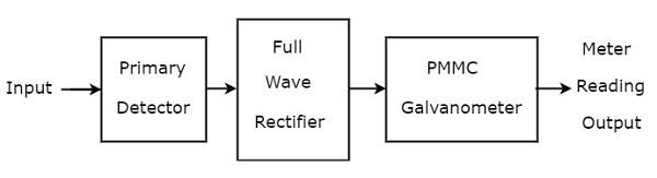
The function of each block present in basic wave analyzer is mentioned below.

• Primary Detector − It consists of an LC circuit. We can adjust the values of inductor, L and capacitor, C in such a way that it allows only the desired harmonic frequency component that is to be measured.

• Full Wave Rectifier − It converts the AC input into a DC output.

• PMMC Galvanometer − It shows the peak value of the signal, which is obtained at the output of Full wave rectifier.

We will get the corresponding circuit diagram, just by replacing each block with the respective component(s) in above block diagram of basic wave analyzer. So, the circuit diagram of basic wave analyzer will look like as shown in the following figure −

This basic wave analyzer can be used for analyzing each and every harmonic frequency component of a periodic signal.

Types of Wave Analyzers

Wave analyzers can be classified into the following two types.

• Frequency Selective Wave Analyzer
• Superheterodyne Wave Analyzer

Now, let us discuss about these two wave analyzers one by one.

Frequency Selective Wave Analyzer

The wave analyzer, used for analyzing the signals are of AF range is called frequency selective wave analyzer. The block diagram of frequency selective wave analyzer is shown in below figure.

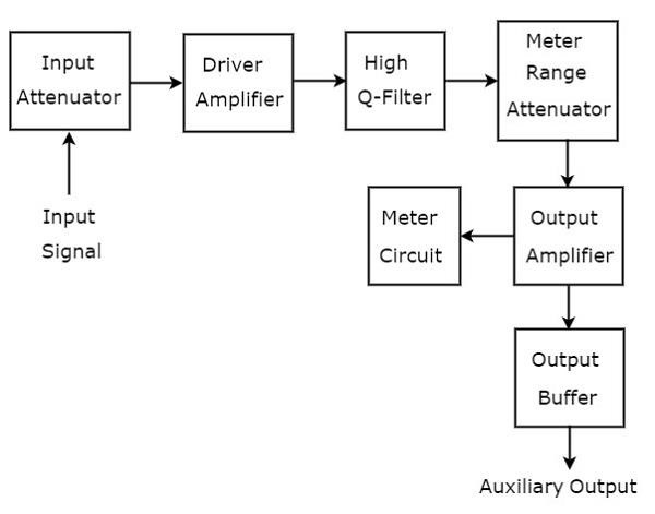
Frequency selective wave analyzer consists a set of blocks. The function of each block is mentioned below.

• Input Attenuator − The AF signal, which is to be analyzed is applied to input attenuator. If the signal amplitude is too large, then it can be attenuated by input attenuator.

• Driver Amplifier − It amplifies the received signal whenever necessary.

• High Q-filter − It is used to select the desired frequency and reject unwanted frequencies. It consists of two RC sections and two filter amplifiers & all these are cascaded with each other. We can vary the capacitance values for changing the range of frequencies in powers of 10. Similarly, we can vary the resistance values in order to change the frequency within a selected range.

• Meter Range Attenuator − It gets the selected AF signal as an input & produces an attenuated output, whenever required.

• Output Amplifier − It amplifies the selected AF signal if necessary.

• Output Buffer − It is used to provide the selected AF signal to output devices.

• Meter Circuit − It displays the reading of selected AF signal. We can choose the meter reading in volt range or decibel range.

Superheterodyne Wave Analyzer

The wave analyzer, used to analyze the signals of RF range is called superheterodyne wave analyzer. The following figure shows the block diagram of superheterodyne wave analyzer.

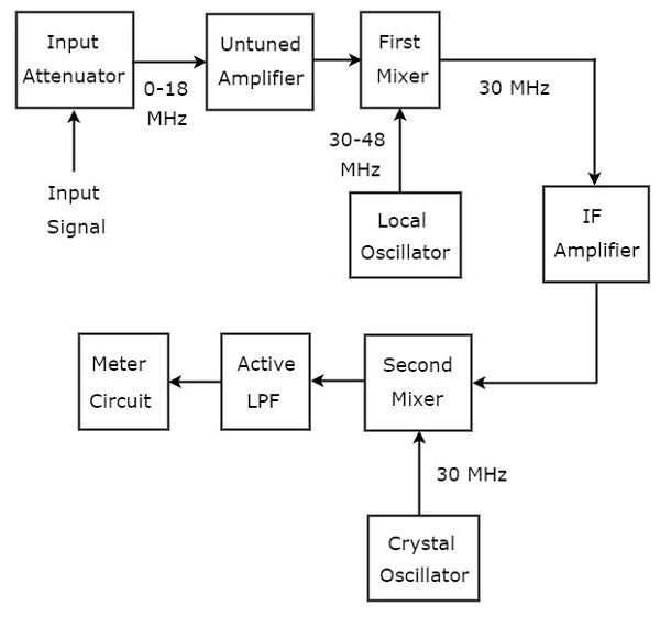
The working of superheterodyne wave analyzer is mentioned below.

• The RF signal, which is to be analyzed is applied to the input attenuator. If the signal amplitude is too large, then it can be attenuated by input attenuator.

• Untuned amplifier amplifies the RF signal whenever necessary and it is applied to first mixer.

• The frequency ranges of RF signal & output of Local oscillator are 0-18 MHz & 30-48 MHz respectively. So, first mixer produces an output, which has frequency of 30 MHz. This is the difference of frequencies of the two signals that are applied to it.

• IF amplifier amplifies the Intermediate Frequency (IF) signal, i.e. the output of first mixer. The amplified IF signal is applied to second mixer.

• The frequencies of amplified IF signal & output of Crystal oscillator are same and equal to 30MHz. So, the second mixer produces an output, which has frequency of 0 Hz. This is the difference of frequencies of the two signals that are applied to it.

• The cut off frequency of Active Low Pass Filter (LPF) is chosen as 1500 Hz. Hence, this filter allows the output signal of second mixer.

• Meter Circuit displays the reading of RF signal. We can choose the meter reading in volt range or decibel range.

So, we can choose a particular wave analyzer based on the frequency range of the signal that is to be analyzed.

Spectrum Analyzers

The electronic instrument, used for analyzing waves in frequency domain is called spectrum analyzer. Basically, it displays the energy distribution of a signal on its CRT screen. Here, x-axis represents frequency and y-axis represents the amplitude.

Types of Spectrum Analyzers

We can classify the spectrum analyzers into the following two types.

• Filter Bank Spectrum Analyzer
• Superheterodyne Spectrum Analyzer

Now, let us discuss about these two spectrum analyzers one by one.

Filter Bank Spectrum Analyzer

The spectrum analyzer, used for analyzing the signals are of AF range is called filter bank spectrum analyzer, or real time spectrum analyzer because it shows (displays) any variations in all input frequencies.

The following figure shows the block diagram of filter bank spectrum analyzer.

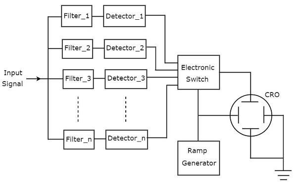
The working of filter bank spectrum analyzer is mentioned below.

• It has a set of band pass filters and each one is designed for allowing a specific band of frequencies. The output of each band pass filter is given to a corresponding detector.

• All the detector outputs are connected to Electronic switch. This switch allows the detector outputs sequentially to the vertical deflection plate of CRO. So, CRO displays the frequency spectrum of AF signal on its CRT screen.

Superheterodyne Spectrum Analyzer

The spectrum analyzer, used for analyzing the signals are of RF range is called superheterodyne spectrum analyzer. Its block diagram is shown in below figure.

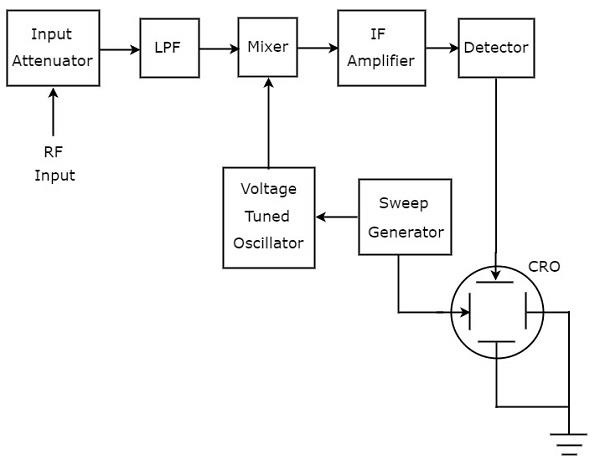
The working of superheterodyne spectrum analyzer is mentioned below.

• The RF signal, which is to be analyzed is applied to input attenuator. If the signal amplitude is too large, then it can be attenuated by an input attenuator.

• Low Pass Filter (LPF) allows only the frequency components that are less than the cut-off frequency.

• Mixer gets the inputs from Low pass filter and voltage tuned oscillator. It produces an output, which is the difference of frequencies of the two signals that are applied to it.

• IF amplifier amplifies the Intermediate Frequency (IF) signal, i.e. the output of mixer. The amplified IF signal is applied to detector.

The output of detector is given to vertical deflection plate of CRO. So, CRO displays the frequency spectrum of RF signal on its CRT screen.

So, we can choose a particular spectrum analyzer based on the frequency range of the signal that is to be analyzed.

Basics of Oscilloscopes

Oscilloscope is an electronic equipment, which displays a voltage waveform. Among the oscilloscopes, Cathode Ray Oscilloscope (CRO) is the basic one and it displays a time varying signal or waveform.

In this chapter, let us discuss about the block diagram of CRO and measurements of some parameters by using CRO.

Block Diagram of CRO

Cathode Ray Oscilloscope (CRO) consists a set of blocks. Those are vertical amplifier, delay line, trigger circuit, time base generator, horizontal amplifier, Cathode Ray Tube (CRT) & power supply. The block diagram of CRO is shown in below figure.

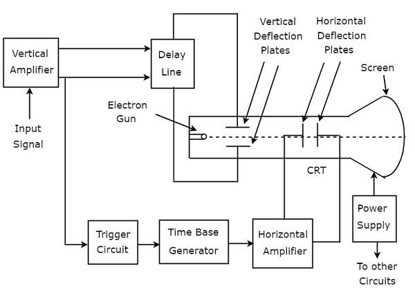
The function of each block of CRO is mentioned below.

• Vertical Amplifier − It amplifies the input signal, which is to be displayed on the screen of CRT.

• Delay Line − It provides some amount of delay to the signal, which is obtained at the output of vertical amplifier. This delayed signal is then applied to vertical deflection plates of CRT.

• Trigger Circuit − It produces a triggering signal in order to synchronize both horizontal and vertical deflections of electron beam.

• Time base Generator − It produces a sawtooth signal, which is useful for horizontal deflection of electron beam.

• Horizontal Amplifier − It amplifies the sawtooth signal and then connects it to the horizontal deflection plates of CRT.

• Power supply − It produces both high and low voltages. The negative high voltage and positive low voltage are applied to CRT and other circuits respectively.

• Cathode Ray Tube (CRT) − It is the major important block of CRO and mainly consists of four parts. Those are electron gun, vertical deflection plates, horizontal deflection plates and fluorescent screen.

The electron beam, which is produced by an electron gun gets deflected in both vertical and horizontal directions by a pair of vertical deflection plates and a pair of horizontal deflection plates respectively. Finally, the deflected beam will appear as a spot on the fluorescent screen.

In this way, CRO will display the applied input signal on the screen of CRT. So, we can analyse the signals in time domain by using CRO

Measurements by using CRO

We can do the following measurements by using CRO.

• Measurement of Amplitude
• Measurement of Time Period
• Measurement of Frequency

Now, let us discuss about these measurements one by one.

Measurement of Amplitude

CRO displays the voltage signal as a function of time on its screen. The amplitude of that voltage signal is constant, but we can vary the number of divisions that cover the voltage signal in vertical direction by varying volt/division knob on the CRO panel. Therefore, we will get the amplitude of the signal, which is present on the screen of CRO by using following formula.

$$A=j\times n_{v}$$

Where,

$A$ is the amplitude

$j$ is the value of volt/division

$n_{v}$ is the number of divisions that cover the signal in vertical direction.

Measurement of Time Period

CRO displays the voltage signal as a function of time on its screen. The Time period of that periodic voltage signal is constant, but we can vary the number of divisions that cover one complete cycle of voltage signal in horizontal direction by varying time/division knob on the CRO panel.

Therefore, we will get the Time period of the signal, which is present on the screen of CRO by using following formula.

$$T=k\times n_{h}$$

Where,

$T$ is the Time period

$j$ is the value of time/division

$n_{v}$ is the number of divisions that cover one complete cycle of the periodic signal in horizontal direction.

Measurement of Frequency

The frequency, f of a periodic signal is the reciprocal of time period, T. Mathematically, it can be represented as

$$f=\frac{1}{T}$$

So, we can find the frequency, f of a periodic signal by following these two steps.

• Step1 − Find the Time period of periodic signal

• Step2 − Take reciprocal of Time period of periodic signal, which is obtained in Step1

We will discuss about special purpose oscilloscopes in next chapter.

Special Purpose Oscilloscopes

In previous chapter, we had discussed about Cathode Ray Oscilloscope (CRO), which is a basic oscilloscope. We will get special purpose oscilloscopes just by including few additional blocks to the basic oscilloscope based on the requirement.

Following are the special purpose oscilloscopes.

• Dual Beam Oscilloscope
• Dual Trace Oscilloscope
• Digital Storage Oscilloscope

Now, let us discuss about these special purpose oscilloscopes one by one.

Dual Beam Oscilloscope

The Oscilloscope, which displays two voltage waveforms is called Dual Beam Oscilloscope. Its block diagram is shown in below figure.

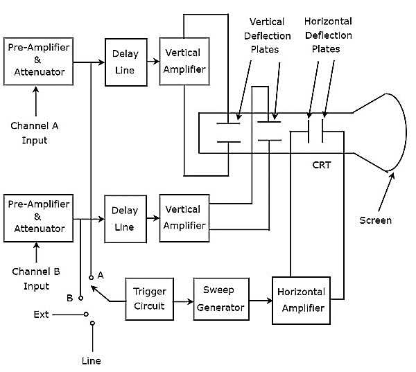
As shown in above figure, the CRT of Dual Beam Oscilloscope consists of two sets of vertical deflection plates and one set of horizontal deflection plates.

The combination of the following blocks together is called a channel.

• Pre-Amplifier & Attenuator
• Delay Line
• Vertical Amplifier
• A set of Vertical Deflection Plates

There are two channels in Dual Beam Oscilloscope. So, we can apply the two signals, namely A & B as input of channel A & Channel B respectively. We can choose any one of these four signals as trigger input to the trigger circuit by using a switch. Those are input signals A & B, External signal (Ext) and Line input.

This oscilloscope will produce two vertically deflected beams, since there are two pairs of vertical deflection plates. In this oscilloscope, the blocks which are useful for deflecting the beam in horizontal direction is common for both the input signals. Finally, this oscilloscope will produce the two input signals simultaneously on the screen of CRT.

Dual Trace Oscilloscope

The Oscilloscope, which produces two traces on its screen is called Dual Trace Oscilloscope. Its block diagram is shown in below figure.

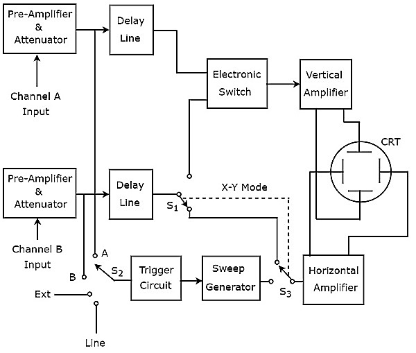
As shown in above figure, the CRT of Dual Trace Oscilloscope consists of a set of vertical deflection plates and another set of horizontal deflection plates. channel consists of four blocks, i.e. pre-Amplifier & attenuator, delay line, vertical amplifier and vertical deflection plates.

In above block diagram, the first two blocks are separately present in both channels. The last two blocks are common to both the channels. Hence, with the help of electronic switch we can connect the delay line output of a specific channel to vertical amplifier.

We can choose any one of these four signals as trigger input to the trigger circuit by using a switch. Those are input signals A & B, External signal (Ext) and Line input.

This oscilloscope uses same electron beam for deflecting the input signals A & B in vertical direction by using an electronic switch, and produces two traces. the blocks that deflect the beam horizontally is common for both the input signals.

Digital Storage Oscilloscope

The oscilloscope, which stores the waveform digitally is known as digital storage oscilloscope. The block diagram of (digital) storage oscilloscope is below −

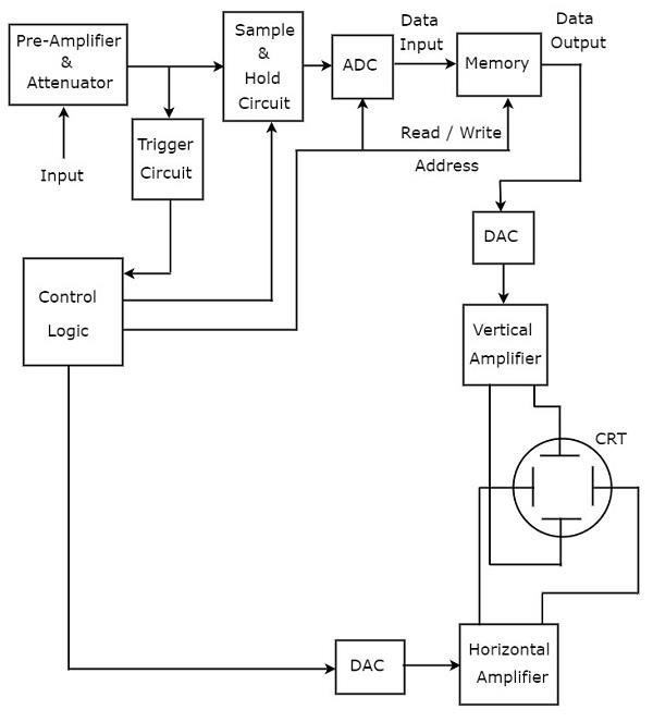
Additional blocks required for digital data storage are added to a basic oscilloscope to make it convert it into a Digital Storage Oscilloscope. The blocks that are required for storing of digital data are lies between the pre-amplifier & attenuator and vertical amplifier in Digital Storage Oscilloscope. Those are Sample and Hold circuit, Analog to Digital Converter (ADC), Memory & Digital to Analog Converter.

Control logic controls the first three blocks by sending various control signals. The blocks like control logic and Digital to Analog Converter are present between the trigger circuit and horizontal amplifier in Digital Storage Oscilloscope.

The Digital Storage Oscilloscope stores the data in digital before it displays the waveform on the screen. Whereas, the basic oscilloscope doesn’t have this feature.

Lissajous Figures

Lissajous figure is the pattern which is displayed on the screen, when sinusoidal signals are applied to both horizontal & vertical deflection plates of CRO. These patterns will vary based on the amplitudes, frequencies and phase differences of the sinusoidal signals, which are applied to both horizontal & vertical deflection plates of CRO.

The following figure shows an example of Lissajous figure.

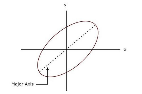
The above Lissajous figure is in elliptical shape and its major axis has some inclination angle with positive x-axis.

Measurements using Lissajous Figures

We can do the following two measurements from a Lissajous figure.

• Frequency of the sinusoidal signal
• Phase difference between two sinusoidal signals

Now, let us discuss about these two measurements one by one.

Measurement of Frequency

Lissajous figure will be displayed on the screen, when the sinusoidal signals are applied to both horizontal & vertical deflection plates of CRO. Hence, apply the sinusoidal signal, which has standard known frequency to the horizontal deflection plates of CRO. Similarly, apply the sinusoidal signal, whose frequency is unknown to the vertical deflection plates of CRO

Let, $f_{H}$ and $f_{V}$ are the frequencies of sinusoidal signals, which are applied to the horizontal & vertical deflection plates of CRO respectively. The relationship between $f_{H}$ and $f_{V}$ can be mathematically represented as below.

$$\frac{f_{V}}{f_{H}}=\frac{n_{H}}{n_{V}}$$

From above relation, we will get the frequency of sinusoidal signal, which is applied to the vertical deflection plates of CRO as

$f_{V}=\left ( \frac{n_{H}}{n_{V}} \right )f_{H}$(Equation 1)

Where,

$n_{H}$ is the number of horizontal tangencies

$n_{V}$ is the number of vertical tangencies

We can find the values of $n_{H}$ and $n_{V}$ from Lissajous figure. So, by substituting the values of $n_{H}$, $n_{V}$ and $f_{H}$ in Equation 1, we will get the value of $f_{V}$, i.e. the frequency of sinusoidal signal that is applied to the vertical deflection plates of CRO.

Measurement of Phase Difference

A Lissajous figure is displayed on the screen when sinusoidal signals are applied to both horizontal & vertical deflection plates of CRO. Hence, apply the sinusoidal signals, which have same amplitude and frequency to both horizontal and vertical deflection plates of CRO.

For few Lissajous figures based on their shape, we can directly tell the phase difference between the two sinusoidal signals.

• If the Lissajous figure is a straight line with an inclination of $45^{\circ}$ with positive x-axis, then the phase difference between the two sinusoidal signals will be $0^{\circ}$. That means, there is no phase difference between those two sinusoidal signals.

• If the Lissajous figure is a straight line with an inclination of $135^{\circ}$ with positive x-axis, then the phase difference between the two sinusoidal signals will be $180^{\circ}$. That means, those two sinusoidal signals are out of phase.

• If the Lissajous figure is in circular shape, then the phase difference between the two sinusoidal signals will be $90^{\circ}$ or $270^{\circ}$.

We can calculate the phase difference between the two sinusoidal signals by using formulae, when the Lissajous figures are of elliptical shape.

• If the major axis of an elliptical shape Lissajous figure having an inclination angle lies between $0^{\circ}$ and $90^{\circ}$ with positive x-axis, then the phase difference between the two sinusoidal signals will be.

$$\phi =\sin ^{-1}\left ( \frac{x_{1}}{x_{2}} \right )=\sin ^{-1}\left ( \frac{y_{1}}{y_{2}} \right )$$

• If the major axis of an elliptical shape Lissajous figure having an inclination angle lies between $90^{\circ}$ and $180^{\circ}$ with positive x-axis, then the phase difference between the two sinusoidal signals will be.

$$\phi =180 - \sin ^{-1}\left ( \frac{x_{1}}{x_{2}} \right )=180 - \sin ^{-1}\left ( \frac{y_{1}}{y_{2}} \right )$$

Where,

$x_{1}$ is the distance from the origin to the point on x-axis, where the elliptical shape Lissajous figure intersects

$x_{2}$ is the distance from the origin to the vertical tangent of elliptical shape Lissajous figure

$y_{1}$ is the distance from the origin to the point on y-axis, where the elliptical shape Lissajous figure intersects

$y_{2}$ is the distance from the origin to the horizontal tangent of elliptical shape Lissajous figure

In this chapter, welearnt how to find the frequency of unknown sinusoidal signal and the phase difference between two sinusoidal signals from Lissajous figures by using formulae.

CRO Probes

We can connect any test circuit to an oscilloscope through a probe. As CRO is a basic oscilloscope, the probe which is connected to it is also called CRO probe.

We should select the probe in such a way that it should not create any loading issues with the test circuit. So that we can analyze the test circuit with the signals properly on CRO screen.

CRO probes should have the following characteristics.

• High impedance
• High bandwidth

The block diagram of CRO probe is shown in below figure.

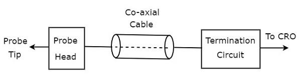
As shown in the figure, CRO probe mainly consists of three blocks. Those are probe head, co-axial cable and termination circuit. Co-axial cable simply connects the probe head and termination circuit.

Types of CRO Probes

CRO probes can be classified into the following two types.

• Passive Probes
• Active Probes

Now, let us discuss about these two types of probes one by one.

Passive Probes

If the probe head consists of passive elements, then it is called passive probe. The circuit diagram of passive probe is shown in below figure.

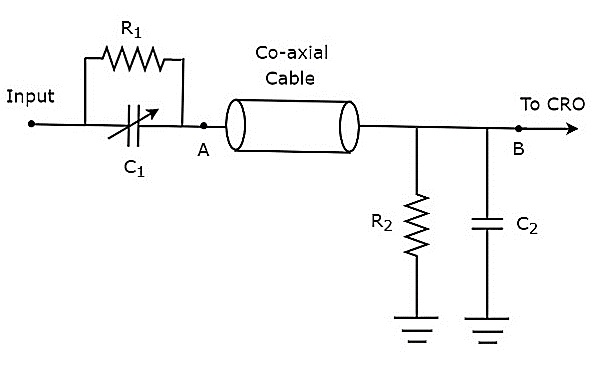
As shown in the figure, the probe head consists of a parallel combination of resistor, $R_{1}$ and a variable capacitor, $C_{1}$. Similarly, the termination circuit consists of a parallel combination of resistor, $R_{2}$ and capacitor, $C_{2}$.

The above circuit diagram is modified in the form of bridge circuit and it is shown in below figure.

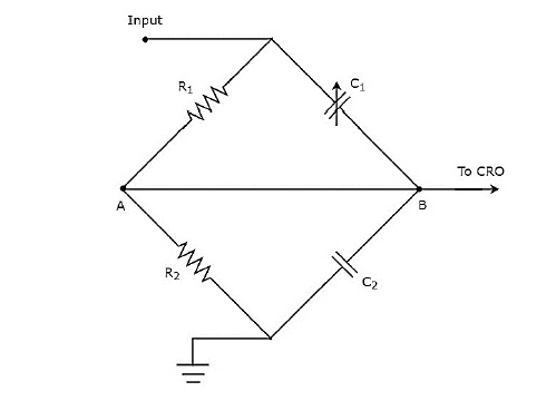
We can balance the bridge, by adjusting the value of variable capacitor, $c_{1}$. We will discuss the concept of bridges in the following chapters. For the time being, consider the following balancing condition of AC bridge.

$$Z_{1}Z_{4}=Z_{2}Z_{3}$$

Substitute, the impedances $Z_{1},Z_{2}, Z_{3}$ and $Z_{4}$ as $R_{1},\frac{1}{j\omega C_{1}}, R_{2}$ and $\frac{1}{j\omega C_{2}}$ respectively in above equation.

$$R_{1}\left ( \frac{1}{j \omega C_{2}} \right )=\left ( \frac{1}{j \omega C_{1}} \right )R_{2}$$

$\Rightarrow R_{1} C_{1}=R_{2} C_{2}$Equation 1

By voltage division principle, we will get the voltage across resistor, $R_{2}$ as

$$V_{0}=V_{i}\left ( \frac{R_{2}}{R_{1}+R_{2}} \right )$$

attenuation factor is the ratio of input voltage, $V_{i}$ and output voltage, $V_{0}$. So, from above equation we will get the attenuation factor, $\alpha$ as

$$\alpha = \frac{V_{i}}{V_{0}}=\frac{R_{1}+R_{2}}{R_{2}}$$

$\Rightarrow \alpha = 1+\frac{R_{1}}{R_{2}}$

$\Rightarrow \alpha-1 = \frac{R_{1}}{R_{2}}$

$\Rightarrow R_{1}= \left ( \alpha-1 \right )R_{2}$Equation 2

From Equation 2, we can conclude that the value of $R_{1}$ is greater than or equal to the value of 𝑅2 for integer values of$\:\alpha > 1$.

Substitute Equation 2 in Equation 1.

$$\left ( \alpha-1 \right )R_{2}C_{1}=R_{2}C_{2}$$

$\Rightarrow \left ( \alpha-1 \right )C_{1} =C_{2}$

$\Rightarrow C_{1}=\frac{C_{2}}{\left ( \alpha-1 \right )}$Equation 3

From Equation 3, we can conclude that the value of $C_{1}$ is less than or equal to the value of $C_{2}$ for integer values of $\alpha >1$

Example

Let us find the values of $R_{1}$ and $C_{1}$ of a probe having an attenuation factor,$\alpha$ as 10. Assume, $R_{2}=1 M \Omega$ and $C_{2}=18pF$.

• Step1 − We will get the value of $R_{1}$ by substituting the values of $\alpha$ and $R_{2}$ in Equation 2.

$$ R_{1}=\left ( 10-1 \right )\times 1 \times 10^{6}$$

$$\Rightarrow R_{1}=9 \times 10^{6}$$

$$\Rightarrow R_{1}=9 M\Omega$$

Step 2 − We will get the value of $C_{1}$ by substituting the values of $\alpha$ and $C_{2}$ in Equation 3.

$$C_{1}=\frac{18\times10^{-12}}{\left ( 10-1 \right )}$$

$$\Rightarrow C_{1}=2 \times 10^{-12}$$

$$\Rightarrow C_{1}=2 pF$$

Therefore, the values of $R_{1}$ and $C_{1}$ of a probe will be $9M\Omega$ and $2pF$ respectively for the given specifications.

Active Probes

If the probe head consists of active electronic components, then it is called active probe. The block diagram of active probe is shown in below figure.

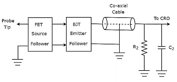
As shown in the figure, the probe head consists of a FET source follower in cascade with BJT emitter follower. The FET source follower provides high input impedance and low output impedance. Whereas, the purpose of BJT emitter follower is that it avoids or eliminates the impedance mismatching.

The other two parts, such as co-axial cable and termination circuit remain same in both active and passive probes.

Electronic Measuring Instruments - Bridges

If the electrical components are arranged in the form a bridge or ring structure, then that electrical circuit is called a bridge. In general, bridge forms a loop with a set of four arms or branches. Each branch may contain one or two electrical components.

Types of Bridges

We can classify the bridge circuits or bridges into the following two categories based on the voltage signal with which those can be operated.

• DC Bridges
• AC Bridges

Now, let us discuss about these two bridges briefly.

DC Bridges

If the bridge circuit can be operated with only DC voltage signal, then it is a DC bridge circuit or simply DC bridge. DC bridges are used to measure the value of unknown resistance. The circuit diagram of DC bridge looks like as shown in below figure.

The above DC bridge has four arms and each arm consists of a resistor. Among which, two resistors have fixed resistance values, one resistor is a variable resistor and the other one has an unknown resistance value.

The above DC bridge circuit can be excited with a DC voltage source by placing it in one diagonal. The galvanometer is placed in other diagonal of DC bridge. It shows some deflection as long as the bridge is unbalanced.

Vary the resistance value of variable resistor until the galvanometer shows null (zero) deflection. Now, the above DC bridge is said to be a balanced one. So, we can find the value of unknown resistance by using nodal equations.

AC Bridges

If the bridge circuit can be operated with only AC voltage signal, then it is said to be AC bridge circuit or simply AC bridge. AC bridges are used to measure the value of unknown inductance, capacitance and frequency.

The circuit diagram of AC bridge looks like as shown in below figure.

The circuit diagram of AC bridge is similar to that of DC bridge. The above AC bridge has four arms and each arm consists of some impedance. That means, each arm will be having either single or combination of passive elements such as resistor, inductor and capacitor.

Among the four impedances, two impedances have fixed values, one impedance is variable and the other one is an unknown impedance.

The above AC bridge circuit can be excited with an AC voltage source by placing it in one diagonal. A detector is placed in other diagonal of AC bridge. It shows some deflection as long as the bridge is unbalanced.

The above AC bridge circuit can be excited with an AC voltage source by placing it in one diagonal. A detector is placed in other diagonal of AC bridge. It shows some deflection as long as the bridge is unbalanced.

Vary the impedance value of variable impedance until the detector shows null (zero) deflection. Now, the above AC bridge is said to be a balanced one. So, we can find the value of unknown impedance by using balanced condition.

DC Bridges

DC bridges can be operated with only DC voltage signal. DC bridges are useful for measuring the value of unknown resistance, which is present in the bridge. Wheatstone’s Bridge is an example of DC bridge.

Now, let us discuss about Wheatstone’s Bridge in order to find the unknown resistance’s value.

Wheatstone’s Bridge

Wheatstone’s bridge is a simple DC bridge, which is mainly having four arms. These four arms form a rhombus or square shape and each arm consists of one resistor.

To find the value of unknown resistance, we need the galvanometer and DC voltage source. Hence, one of these two are placed in one diagonal of Wheatstone’s bridge and the other one is placed in another diagonal of Wheatstone’s bridge.

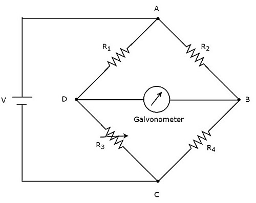
Wheatstone’s bridge is used to measure the value of medium resistance. The circuit diagram of Wheatstone’s bridge is shown in below figure.

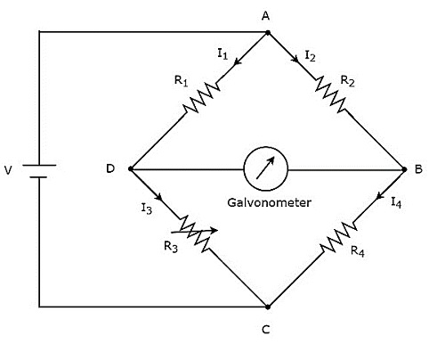
In above circuit, the arms AB, BC, CD and DA together form a rhombus or square shape. They consist of resistors $R_{2}$, $R_{4}$, $R_{3}$ and $R_{1}$ respectively. Let the current flowing through these resistor arms is $I_{2}$, $I_{4}$, $I_{3}$ and $I_{1}$ respectively and the directions of these currents are shown in the figure.

The diagonal arms DB and AC consists of galvanometer and DC voltage source of V volts respectively. Here, the resistor, $R_{3}$ is a standard variable resistor and the resistor, $R_{4}$ is an unknown resistor. We can balance the bridge, by varying the resistance value of resistor, $R_{3}$.

The above bridge circuit is balanced when no current flows through the diagonal arm, DB. That means, there is no deflection in the galvanometer, when the bridge is balanced.

The bridge will be balanced, when the following two conditions are satisfied.

• The voltage across arm AD is equal to the voltage across arm AB. i.e.,

$$V_{AD}=V_{AB}$$

$\Rightarrow I_{1}R_{1}=I_{2}R_{2}$Equation 1

• The voltage across arm DC is equal to the voltage across arm BC. i.e.,

$$V_{DC}=V_{BC}$$

$\Rightarrow I_{3}R_{3}=I_{4}R_{4}$Equation 2

From above two balancing conditions, we will get the following two conclusions.

• The current flowing through the arm AD will be equal to that of arm DC. i.e.,

$$I_{1}=I_{3}$$

• The current flowing through the arm AB will be equal to that of arm BC. i.e.,

$$I_{2}=I_{4}$$

Take the ratio of Equation 1 and Equation 2.

$\frac{I_{1}R_{1}}{I_{3}R_{3}}=\frac{I_{2}R_{2}}{I_{4}R_{4}}$Equation 3

Substitute, $I_{1}=I_{3}$ and $I_{2}=I_{4}$ in Equation 3.

$$\frac{I_{3}R_{1}}{I_{3}R_{3}}=\frac{I_{4}R_{2}}{I_{4}R_{4}}$$

$$\Rightarrow \frac{R_{1}}{R_{3}}=\frac{R_{2}}{R_{4}}$$

$$\Rightarrow R_{4}=\frac{R_{2}R_{3}}{R_{1}}$$

By substituting the known values of resistors $R_{1}$, $R_{2}$ and $R_{3}$ in above equation, we will get the value of resistor,$R_{4}$.

AC Bridges

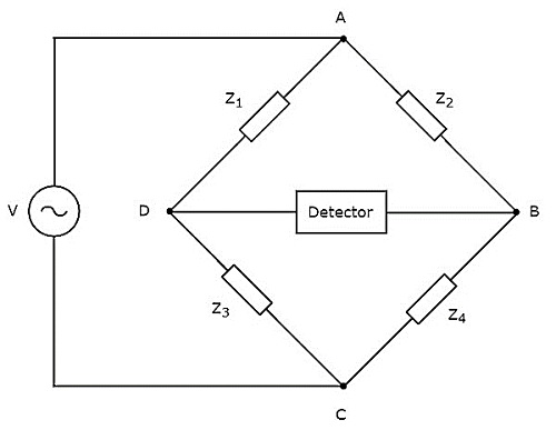
In this chapter, let us discuss about the AC bridges, which can be used to measure inductance. AC bridges operate with only AC voltage signal. The circuit diagram of AC bridge is shown in below figure.

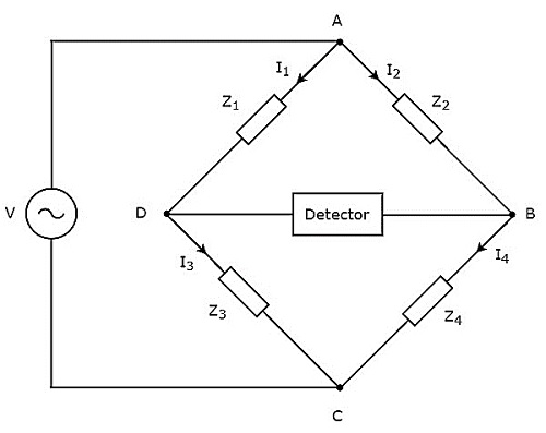
As shown in above figure, AC bridge mainly consists of four arms, which are connected in rhombus or square shape. All these arms consist of some impedance.

The detector and AC voltage source are also required in order to find the value of unknown impedance. Hence, one of these two are placed in one diagonal of AC bridge and the other one is placed in other diagonal of AC bridge. The balancing condition of Wheatstone’s bridge as −

$$R_{4}=\frac{R_{2}R_{3}}{R_{1}}$$

We will get the balancing condition of AC bridge, just by replacing R with Z in above equation.

$$Z_{4}=\frac{Z_{2}Z_{3}}{Z_{1}}$$

$\Rightarrow Z_{1}Z_{4}=Z_{2}Z_{3}$

Here, $Z_{1}$ and $Z_{2}$ are fixed impedances. Whereas, $Z_{3}$ is a standard variable impedance and $Z_{4}$ is an unknown impedance.

Note − We can choose any two of those four impedances as fixed impedances, one impedance as standard variable impedance & the other impedance as an unknown impedance based on the application.

Following are the two AC bridges, which can be used to measure inductance.

• Maxwell’s Bridge
• Hay’s Bridge

Now, let us discuss about these two AC bridges one by one.

Maxwell's Bridge

Maxwell’s bridge is an AC bridge having four arms, which are connected in the form of a rhombus or square shape. Two arms of this bridge consist of a single resistor, one arm consists of a series combination of resistor and inductor & the other arm consists of a parallel combination of resistor and capacitor.

An AC detector and AC voltage source are used to find the value of unknown impedance. Hence, one of these two are placed in one diagonal of Maxwell’s bridge and the other one is placed in other diagonal of Maxwell’s bridge.

Maxwell’s bridge is used to measure the value of medium inductance. The circuit diagram of Maxwell’s bridge is shown in the below figure.

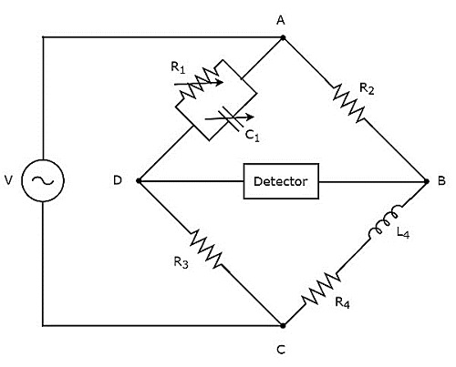
In above circuit, the arms AB, BC, CD and DA together form a rhombus or square shape. The arms AB and CD consist of resistors, $R_{2}$ and $R_{3}$ respectively. The arm, BC consists of a series combination of resistor, $R_{4}$ and inductor, $L_{4}$. The arm, DA consists of a parallel combination of resistor, $R_{1}$ and capacitor, $C_{1}$.

Let, $Z_{1}, Z_{2}, Z_{3}$ and $Z_{4}$ are the impedances of arms DA, AB, CD and BC respectively. The values of these impedances will be

$$Z_{1}=\frac{R_{1}\left ( \frac{1}{j\omega C_{1}} \right )}{R_{1}+\frac{1}{j\omega C_{1}}}$$

$$\Rightarrow Z_{1}=\frac{R_{1}}{1+j \omega R_{1}C_{1}}$$

$Z_{2}=R_{2}$

$Z_{3}=R_{3}$

$Z_{4}=R_{4}+j \omega L_{4}$

Substitute these impedance values in the following balancing condition of AC bridge.

$$Z_{4}=\frac{Z_{2}Z_{3}}{Z_{1}}$$

$$R_{4}+j\omega L_{4}=\frac{R_{2}R_{3}}{\left ( {\frac{R_{1}}{1+j \omega R_{1}C_{1}}} \right )}$$

$\Rightarrow R_{4}+j\omega L_{4}=\frac{R_{2}R_{3}\left (1+j \omega R_{1}C_{1} \right )}{R_{1}}$

$\Rightarrow R_{4}+j\omega L_{4}=\frac{R_{2}R_{3}}{R_{1}}+\frac{j \omega R_{1}C_{1}R_{2}R_{3}}{R_{1}}$

$\Rightarrow R_{4}+j\omega L_{4}=\frac{R_{2}R_{3}}{R_{1}}+j \omega C_{1}R_{2}R_{3}$

By comparing the respective real and imaginary terms of above equation, we will get

$R_{4}=\frac{R_{2}R_{3}}{R_{1}}$Equation 1

$L_{4}=C_{1}R_{2}R_{3}$Equation 2

By substituting the values of resistors $R_{1}$, $R_{2}$ and $R_{3}$ in Equation 1, we will get the value of resistor, $R_{4}$. Similarly, by substituting the value of capacitor, $C_{1}$ and the values of resistors, $R_{2}$ and $R_{3}$ in Equation 2, we will get the value of inductor, $L_{4}$.

The advantage of Maxwell’s bridge is that both the values of resistor, $R_{4}$ and an inductor, $L_{4}$ are independent of the value of frequency.

Hay’s Bridge

Hay’s bridge is a modified version of Maxwell’s bridge, which we get by modifying the arm, which consists of a parallel combination of resistor and capacitor into the arm, which consists of a series combination of resistor and capacitor in Maxwell’s bridge.

Hay’s bridge is used to measure the value of high inductance. The circuit diagram of Hay’s bridge is shown in the below figure.

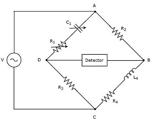
In above circuit, the arms AB, BC, CD and DA together form a rhombus or square shape. The arms, AB and CD consist of resistors, $R_{2}$ and $R_{3}$ respectively. The arm, BC consists of a series combination of resistor, $R_{4}$ and inductor, $L_{4}$. The arm, DA consists of a series combination of resistor, $R_{1}$ and capacitor, $C_{1}$.

Let, $Z_{1}, Z_{2}, Z_{3}$ and $Z_{4}$ are the impedances of arms DA, AB, CD and BC respectively. The values of these impedances will be

$$Z_{1}=R_{1}+\frac{1}{j \omega C_{1}}$$

$\Rightarrow Z_{1}=\frac{1+j \omega R_{1}C_{1}}{j \omega C_{1}}$

$Z_{2}=R_{2}$

$Z_{3}=R_{3}$

$Z_{4}=R_{4}+j \omega L_{4}$

Substitute these impedance values in the following balancing condition of AC bridge.

$$Z_{4}=\frac{Z_{2}Z_{3}}{Z_{1}}$$

$R_{4}+j \omega L_{4}=\frac{R_{2}R_{3}}{\left ( \frac{1+j \omega R_{1}C_{1}}{j \omega C_{1}}\right )}$

$R_{4}+j \omega L_{4}=\frac{R_{2}R_{3}j \omega C_{1}}{\left ( 1+j \omega R_{1}C_{1}\right )}$

Multiply the numerator and denominator of right hand side term of above equation with $1 - j \omega R_{1}C_{1}$.

$\Rightarrow R_{4}+j \omega L_{4}=\frac{R_{2}R_{3}j \omega C_{1}}{\left ( 1+j \omega R_{1}C_{1}\right )}\times \frac{\left (1 - j \omega R_{1}C_{1} \right )}{\left (1 - j \omega R_{1}C_{1} \right )}$

$\Rightarrow R_{4}+j \omega L_{4}=\frac{\omega^{2}{C_{1}}^{2}R_{1}R_{2}R_{3}+j \omega R_{2}R_{3}C_{1}}{\left ( 1+\omega^{2}{R_{1}}^{2}{C_{1}}^{2}\right )}$

By comparing the respective real and imaginary terms of above equation, we will get

$R_{4}= \frac{\omega^{2}{C_{1}}^{2}R_{1}R_{2}R_{3}}{\left ( 1+\omega^{2}{R_{1}}^{2}{C_{1}}^{2}\right )}$Equation 3

$L_{4}= \frac{R_{2}R_{3}C_{1}}{\left ( 1+\omega^{2}{R_{1}}^{2}{C_{1}}^{2}\right )}$Equation 4

By substituting the values of $R_{1}, R_{2}, R_{3}, C_{1}$ and $\omega$ in Equation 3 and Equation 4, we will get the values of resistor, $R_{4}$ and inductor, $L_{4}$.

Other AC Bridges

In previous chapter, we discussed about two AC bridges which can be used to measure inductance. In this chapter, let us discuss about the following two AC bridges.

• Schering Bridge
• Wien’s Bridge

These two bridges can be used to measure capacitance and frequency respectively.

Schering Bridge

Schering bridge is an AC bridge having four arms, which are connected in the form of a rhombus or square shape, whose one arm consists of a single resistor, one arm consists of a series combination of resistor and capacitor, one arm consists of a single capacitor & the other arm consists of a parallel combination of resistor and capacitor.

The AC detector and AC voltage source are also used to find the value of unknown impedance, hence one of them is placed in one diagonal of Schering bridge and the other one is placed in other diagonal of Schering bridge.

Schering bridge is used to measure the value of capacitance. The circuit diagram of Schering bridge is shown in the below figure.

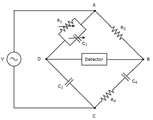
In above circuit, the arms AB, BC, CD and DA together form a rhombus or square shape. The arm AB consists of a resistor, $R_{2}$. The arm BC consists of a series combination of resistor, $R_{4}$ and capacitor, $C_{4}$. The arm CD consists of a capacitor, $C_{3}$. The arm DA consists of a parallel combination of resistor, $R_{1}$ and capacitor, $C_{1}$.

Let, $Z_{1}$, $Z_{2}$,$Z_{3}$ and $Z_{4}$ are the impedances of arms DA, AB, CD and BC respectively. The values of these impedances will be

$Z_{1}=\frac{R_{1}\left ( \frac{1}{j \omega C_{1}} \right )}{R_{1}+\frac{1}{j \omega C_{1}}}$

$\Rightarrow Z_{1}=\frac{R_{1}}{1+j \omega R_{1}C_{1}}$

$Z_{2}=R_{2}$

$Z_{3}=\frac{1}{j \omega C_{3}}$

$Z_{4}=R_{4}+\frac{1}{j \omega C_{4}}$

$\Rightarrow Z_{4}=\frac{1+j \omega R_{4}C_{4}}{j \omega C_{4}}$

Substitute these impedance values in the following balancing condition of AC bridge.

$$Z_{4}=\frac{Z_{2}Z_{3}}{Z_{1}}$$

$$\frac{1+j \omega R_{4}C_{4}}{j \omega C_{4}}=\frac{R_{2}\left (\frac{1}{j \omega C_{3}} \right )}{\frac{R_{1}}{1+j \omega R_{1}C_{1}}}$$

$\Rightarrow \frac{1+j \omega R_{4}C_{4}}{j \omega C_{4}}=\frac{R_{2}\left ( 1+j \omega R_{1}C_{1} \right )}{j \omega R_{1}C_{3}}$

$\Rightarrow \frac{1+j \omega R_{4}C_{4}}{C_{4}}=\frac{R_{2}\left ( 1+j \omega R_{1}C_{1} \right )}{R_{1}C_{3}}$

$\Rightarrow \frac{1}{C_{4}}+j \omega R_{4}=\frac{R_{2}}{R_{1}C_{3}}+\frac{j\omega C_{1}R_{2}}{C_{3}}$

By comparing the respective real and imaginary terms of above equation, we will get

$C_{4}=\frac{R_{1}C_{3}}{R_{2}}$Equation 1

$R_{4}=\frac{C_{1}R_{2}}{C_{3}}$Equation 2

By substituting the values of $R_{1}, R_{2}$ and $C_{3}$ in Equation 1, we will get the value of capacitor, $C_{4}$. Similarly, by substituting the values of $R_{2}, C_{1}$ and $C_{3}$ in Equation 2, we will get the value of resistor, $R_{4}$.

The advantage of Schering bridge is that both the values of resistor, $R_{4}$ and capacitor, $C_{4}$ are independent of the value of frequency.

Wien’s Bridge

Wien’s bridge is an AC bridge having four arms, which are connected in the form of a rhombus or square shape. Amongtwo arms consist of a single resistor, one arm consists of a parallel combination of resistor and capacitor & the other arm consists of a series combination of resistor and capacitor.

The AC detector and AC voltage source are also required in order to find the value of frequency. Hence, one of these two are placed in one diagonal of Wien’s bridge and the other one is placed in other diagonal of Wien’s bridge.

The circuit diagram of Wien’s bridge is shown in the below figure.

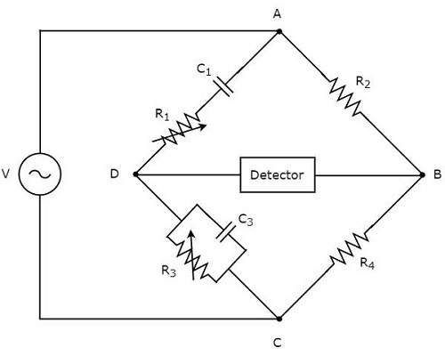
In above circuit, the arms AB, BC, CD and DA together form a rhombus or square shape. The arms, AB and BC consist of resistors, $R_{2}$ and $R_{4}$ respectively. The arm, CD consists of a parallel combination of resistor, $R_{3}$ and capacitor, $C_{3}$. The arm, DA consists of a series combination of resistor, $R_{1}$ and capacitor, $C_{1}$.

Let, $Z_{1}, Z_{2}, Z_{3}$ and $Z_{4}$ are the impedances of arms DA, AB, CD and BC respectively. The values of these impedances will be

$$Z_{1}=R_{1}+\frac{1}{j \omega C_{1}}$$

$$\Rightarrow Z_{1}=\frac{1+j \omega R_{1}C_{1}}{j \omega C_{1}}$$

$Z_{2}=R_{2}$

$$Z_{3}=\frac{R_{3}\left (\frac{1}{j \omega C_{3}} \right )}{R_{3}+\frac{1}{j \omega C_{3}}}$$

$$\Rightarrow Z_{3}= \frac{R_{3}}{1+j \omega R_{3}C_{3}}$$

$Z_{4}=R_{4}$

Substitute these impedance values in the following balancing condition of AC bridge.

$$Z_{1}Z_{4}=Z_{2}Z_{3}$$

$$\left (\frac{1+j \omega R_{1}C_{1}}{j \omega C_{1}} \right )R_{4}=R_{2}\left (\frac{R_{3}}{1+j \omega R_{3}C_{3}} \right )$$

$\Rightarrow \left (1+j \omega R_{1}C_{1}\right )\left (1+j \omega R_{3}C_{3}\right )R_{4}=j \omega C_{1}R_{2}R_{3}$

$\Rightarrow \left (1+j \omega R_{3}C_{3}+j \omega R_{1}C_{1}-\omega^{2}R_{1}R_{3}C_{1}C_{3}\right )R_{4}=j \omega C_{1}R_{2}R_{3}$

$\Rightarrow R_{4}\left ( \omega^{2}R_{1}R_{3}C_{1}C_{3} \right )+j \omega R_{4}\left (R_{3}C_{3}+R_{1}C_{1} \right )=j \omega C_{1}R_{2}R_{3}$

Equate the respective real terms of above equation.

$$R_{4}\left (1- \omega^{2}R_{1}R_{3}C_{1}C_{3} \right )=0$$

$\Rightarrow 1- \omega^{2}R_{1}R_{3}C_{1}C_{3} =0$

$\Rightarrow 1= \omega^{2}R_{1}R_{3}C_{1}C_{3}$

$\omega = \frac{1}{\sqrt{R_{1}R_{3}C_{1}C_{3}}}$

Substitute, $\omega = 2 \pi f$ in above equation.

$$\Rightarrow 2 \pi f= \frac{1}{\sqrt{R_{1}R_{3}C_{1}C_{3}}}$$

$\Rightarrow f= \frac{1}{2 \pi\sqrt{R_{1}R_{3}C_{1}C_{3}}}$

We can find the value of frequency, $f$ of AC voltage source by substituting the values of $R_{1}, R_{3}, C_{1}$ and $C_{3}$ in above equation.

If $R_{1}=R_{3}=R$ and $C_{1}=C_{3}=C$, then we can find the value of frequency, $f$ of AC voltage source by using the following formula.

$$f=\frac{1}{2\pi RC}$$

The Wein’s bridge is mainly used for finding the frequency value of AF range.

Transducers

Basically, Transducer converts one form of energy into another form of energy. The transducer, which converts non-electrical form of energy into electrical form of energy is known as electrical transducer. The block diagram of electrical transducer is shown in below figure.

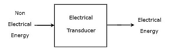
As shown in the figure, electrical transducer will produce an output, which has electrical energy. The output of electrical transducer is equivalent to the input, which has non-electrical energy.

Types of Electrical Transducers

Mainly, the electrical transducers can be classified into the following two types.

• Active Transducers
• Passive Transducers

Now, let us discuss about these two types of transducers briefly.

Active Transducers

The transducer, which can produce one of the electrical quantities such as voltage and current is known as active transducer. It is also called self-generating transducer, since it doesn’t require any external power supply.

The block diagram of active transducer is shown in below figure.

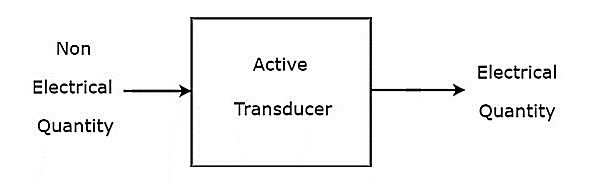
As shown in the figure, active transducer will produce an electrical quantity (or signal), which is equivalent to the non-electrical input quantity (or signal).

Examples

Following are the examples of active transducers.

• Piezo Electric Transducer
• Photo Electric Transducer
• Thermo Electric Transducer

We will discuss about these active transducers in next chapter.

Passive Transducers

The transducer, which can’t produce the electrical quantities such as voltage and current is known as passive transducer. But, it produces the variation in one of passive elements like resistor (R), inductor (L) and capacitor (C). Passive transducer requires external power supply.

The block diagram of passive transducer is shown in below figure.

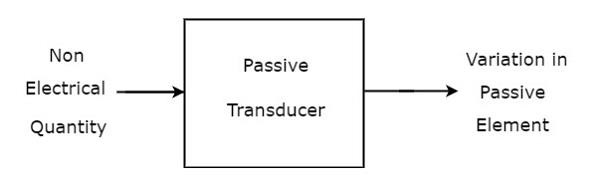
As shown in the figure, passive transducer will produce variation in the passive element in accordance with the variation in the non-electrical input quantity (or signal).

Examples

Following are the examples of passive transducers.

• Resistive Transducer
• Inductive Transducer
• Capacitive Transducer

We will discuss about these passive transducers in later chapters.

Active Transducers

Active transducer is a transducer, which converts the non-electrical quantity into an electrical quantity. Let us consider the non-electrical quantities such as pressure, illumination of light and temperature. Hence, we will get the following three active transducers depending on the non-electrical quantity that we choose.

• Piezo Electric Transducer
• Photo Electric Transducer
• Thermo Electric Transducer

Now, let us discuss about these three active transducers one by one.

Piezo Electric Transducer

An active transducer is said to be piezo electric transducer, when it produces an electrical quantity which is equivalent to the pressure input. The following three substances exhibit piezo electric effect.

• Quartz
• Rochelle salts
• Tourmaline

The piezo-electric effect exhibited by these three substances is Tourmaline, Quartz, and Rochelle salts, in this ascending order. The ascending order of mechanical strength having by these three substances is Rochelle salts, Quartz, Tourmaline.

Quartz is used as piezo electric transducer, as it exhibits the moderate piezo electric effect and having moderate mechanical strength among those three piezo electric substances.

Quartz Transducer

The circuit diagram of Quartz transducer is shown in below figure. As shown in the figure, quartz crystal is placed between base and force summing member. The output voltage can be measured across the metal electrodes, which are placed on two sides of quartz crystal.

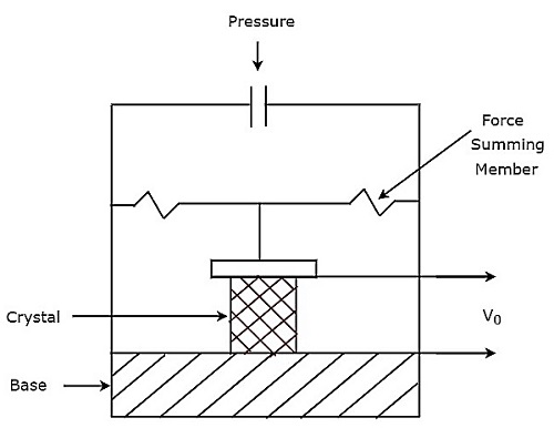
The output voltage, $V_{0}$ of above pressure transducer will be

$$V_{0}=\frac{Q}{C}$$

Photo Electric Transducer

An active transducer is said to be photo electric transducer, when it produces an electrical quantity which is equivalent to the illumination of light input. The circuit diagram of photo electric transducer is shown in below figure.

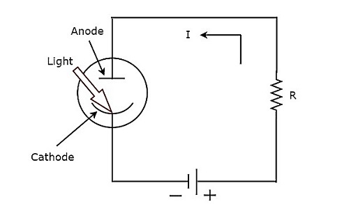
The working of photo electric transducer is mentioned below.

• Step1 − The photo electric transducer releases electrons, when the light falls on cathode of it.

• Step2 − The photo electric transducer produces a current, I in the circuit due to the attraction of electrons towards anode.

We can find the sensitivity of photo electric transducer by using the following formula.

$$S=\frac{I}{i}$$

Where,

$S$ is the sensitivity of photo electric transducer

$I$ is the output current of photo electric transducer

$i$ is the illumination of the light input of photo electric transducer

Thermo Electric Transducer

An active transducer is said to be thermo electric transducer, when it produces an electrical quantity which is equivalent to temperature input. The following two transducers are the examples of thermo electric transducers.

• Thermistor Transducer
• Thermocouple Transducer

Now, let us discuss about these two transducers one by one.

Thermistor Transducer

The resistor, which depends on temperature is called thermal resistor. In short, it is called Thermistor. The temperature coefficient of thermistor is negative. That means, as temperature increases, the resistance of thermistor decreases.

Mathematically, the relation between resistance of thermistor and temperature can be represented as

$$R_{1}=R_{2}e^\left ( \beta \left [ \frac{1}{T_{1}}-\frac{1}{T_{2}} \right ] \right )$$

Where,

$R_{1}$ is the resistance of thermistor at temperature ${T_{1}}^{0}K$

$R_{2}$ is the resistance of thermistor at temperature ${T_{2}}^{0}K$

$\beta$ is the temperature constant

The advantage of Thermistor transducer is that it will produce a fast and stable response.

Thermocouple Transducer

Thermocouple transducer produces an output voltage for a corresponding change of temperature at the input. If two wires of different metals are joined together in order to create two junctions, then that entire configuration is called Thermocouple. The circuit diagram of basic thermocouple is shown below −

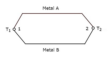
The above thermocouple has two metals, A & B and two junctions, 1 & 2. Consider a constant reference temperature, $T_{2}$ at junction 2. Let the temperature at junction, 1 is $T_{1}$. Thermocouple generates an emf (electro motive force), whenever the values of $T_{1}$ and $T_{2}$ are different.

That means, thermocouple generates an emf, whenever there is a temperature difference between the two junctions, 1 & 2 and it is directly proportional to the temperature difference between those two junctions. Mathematically, it can be represented as

$$e \alpha \left ( T_{1}-T_{2} \right )$$

Where,

$e$ is the emf generated by thermocouple

The above thermocouple circuit can be represented as shown in below figure for practical applications.

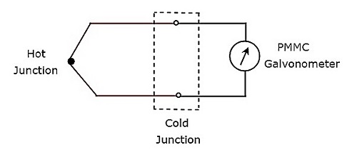
The part of the circuit, which lies between hot & cold junctions including those two junctions is an equivalent model of basic thermocouple. A PMMC galvanometer is connected across the cold junction and it deflects according to the emf generated across cold junction. Thermocouple transducer is the most commonly used thermoelectric transducer.

Passive Transducers

passive transducer is a transducer, which produces the variation in passive element. We will consider the passive elements like resistor, inductor and capacitor. Hence, we will get the following three passive transducers depending on the passive element that we choose.

• Resistive Transducer
• Inductive Transducer
• Capacitive Transducer

Now, let us discuss about these three passive transducers one by one.

Resistive Transducer

A passive transducer is said to be a resistive transducer, when it produces the variation (change) in resistance value. the following formula for resistance, R of a metal conductor.

$$R=\frac{\rho \:l}{A}$$

Where,

$\rho$ is the resistivity of conductor

$l$ is the length of conductor

$A$ is the cross sectional area of the conductor

The resistance value depends on the three parameters $\rho, l$ & $A$. So, we can make the resistive transducers based on the variation in one of the three parameters $\rho, l$ & $A$. The variation in any one of those three parameters changes the resistance value.

• Resistance, R is directly proportional to the resistivity of conductor, $\rho$. So, as resistivity of conductor, $\rho$ increases the value of resistance, R also increases. Similarly, as resistivity of conductor, $\rho$ decreases the value of resistance, R also decreases.

• Resistance, R is directly proportional to the length of conductor, $l$. So, as length of conductor, $l$ increases the value of resistance, R also increases. Similarly, as length of conductor, $l$ decreases the value of resistance, R also decreases.

• Resistance, R is inversely proportional to the cross sectional area of the conductor, $A$. So, as cross sectional area of the conductor, $A$ increases the value of resistance, R decreases. Similarly, as cross sectional area of the conductor, $A$ decreases the value of resistance, R increases.

Inductive Transducer

A passive transducer is said to be an inductive transducer, when it produces the variation (change) in inductance value. the following formula for inductance, L of an inductor.

$L=\frac{N^{2}}{S}$Equation 1

Where,

$N$ is the number of turns of coil

$S$ is the number of turns of coil

the following formula for reluctance, S of coil.

$S=\frac{l}{\mu A}$Equation 2

Where,

$l$ is the length of magnetic circuit

$\mu$ is the permeability of core

$A$ is the area of magnetic circuit through which flux flows

Substitute, Equation 2 in Equation 1.

$$L=\frac{N^{2}}{\left (\frac{l}{\mu A} \right )}$$

$\Rightarrow L=\frac{N^{2}\mu A}{l}$Equation 3

From Equation 1 & Equation 3, we can conclude that the inductance value depends on the three parameters $N,S$ & $\mu$. So, we can make the inductive transducers based on the variation in one of the three parameters $N,S$ & $\mu$. Because, the variation in any one of those three parameters changes the inductance value.

• Inductance, L is directly proportional to square of the number of turns of coil. So, as number of turns of coil, $N$ increases the value of inductance, $L$ also increases. Similarly, as number of turns of coil, $N$ decreases the value of inductance, $L$ also decreases.

• Inductance, $L$ is inversely proportional to reluctance of coil, $S$. So, as reluctance of coil, $S$ increases the value of inductance, $L$ decreases. Similarly, as reluctance of coil, $S$ decreases the value of inductance, $L$ increases.

• Inductance, L is directly proportional to permeability of core, $\mu$. So, as permeability of core, $\mu$ increases the value of inductance, L also increases. Similarly, as permeability of core, $\mu$ decreases the value of inductance, L also decreases.

Capacitive Transducer

A passive transducer is said to be a capacitive transducer, when it produces the variation (change) in capacitance value. the following formula for capacitance, C of a parallel plate capacitor.

$$C=\frac{\varepsilon A}{d}$$

Where,

$\varepsilon$ is the permittivity or the dielectric constant

$A$ is the effective area of two plates

$d$ is the effective area of two plates

The capacitance value depends on the three parameters $\varepsilon, A$ & $d$. So, we can make the capacitive transducers based on the variation in one of the three parameters$\varepsilon, A$ & $d$. Because, the variation in any one of those three parameters changes the capacitance value.

• Capacitance, C is directly proportional to permittivity, $\varepsilon$. So, as permittivity, $\varepsilon$ increases the value of capacitance, C also increases. Similarly, as permittivity, $\varepsilon$ decreases the value of capacitance, C also decreases.

• Capacitance, C is directly proportional to the effective area of two plates, $A$. So, as effective area of two plates, $A$ increases the value of capacitance, C also increases. Similarly, as effective area of two plates, $A$ decreases the value of capacitance, C also decreases.

• Capacitance, C is inversely proportional to the distance between two plates, $d$. So, as distance between two plates, $d$ increases the value of capacitance, C decreases. Similarly, as distance between two plates, $d$ decreases the value of capacitance, C increases.

In this chapter, we discussed about three passive transducers. In next chapter, let us discuss about an example for each passive transducer.

Measurement Of Displacement

The physical quantities such as displacement, velocity, force, temperature & etc. are all non-electrical quantities. active transducer converts the physical quantity into an electrical signal. Whereas, passive transducer converts the physical quantity into the variation in passive element.

So, based on the requirement we can choose either active transducer or passive transducer. In this chapter, let us discuss how to measure displacement by using a passive transducer. If a body that moves from one point to another point in a straight line, then the length between those two points is called displacement.

We have the following three passive transducers

• Resistive Transducer
• Inductive Transducer
• Capacitive Transducer

Now, let us discuss about the measurement of displacement with these three passive transducers one by one.

Measurement of Displacement using Resistive Transducer

The circuit diagram of resistive transducer, which is used to measure displacement is shown in below figure.

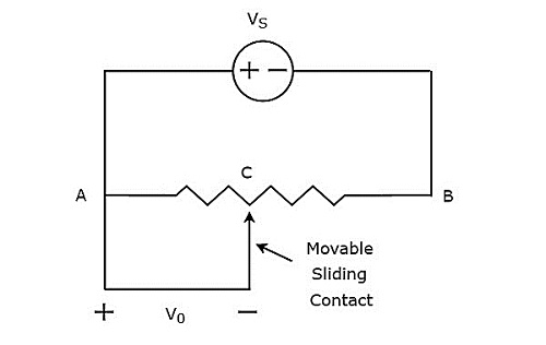
The above circuit consists of a potentiometer and a voltage source, $V_{S}$. We can say that these two are connected in parallel with respect to the points A & B. Potentiometer has a sliding contact, which can be varied. So, the point C is a variable one. In above circuit, the output voltage, $V_{0}$ is measured across the points A & C.

Mathematically, the relation between the voltages and distances can be represented as

$$\frac{V_{0}}{V_{S}}=\frac{AC}{AB}$$

Therefore, we should connect the body whose displacement is to be measured to the sliding contact. So, whenever the body moves in a straight line, the point C also varies. Due to this, the output voltage, $V_{0}$ also changes accordingly.

In this case, we can find the displacement by measuring the output voltage, $V_{0}$.

Measurement of Displacement using Inductive Transducer

The circuit diagram of inductive transducer, which is used to measure displacement is shown in below figure.

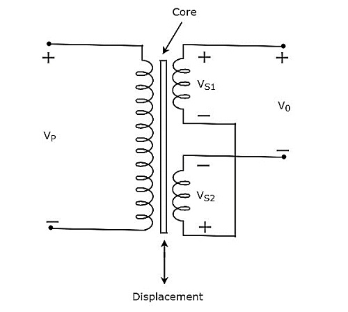
The transformer present in above circuit has a primary winding and two secondary windings. Here, the ending points of two secondary windings are joined together. So, we can say that these two secondary windings are connected in series opposition.

The voltage, $V_{P}$ is applied across the primary winding of transformer. Let, the voltage developed across each secondary winding is 𝑉𝑆1 and 𝑉𝑆2. The output voltage, $V_{0}$ is taken across the starting points of two secondary windings.

Mathematically, the output voltage, 𝑉0 can be written as

$$V_{0}= V_{S1}-V_{S2}$$

The transformer present in above circuit is called differential transformer, since it produces an output voltage, which is the difference between $V_{S1}$ and $V_{S2}$.

• If the core is at central position, then the output voltage, $V_{0}$ will be equal to zero. Because, the respective magnitudes & phases of $V_{S1}$ and $V_{S2}$ are same.

• If the core is not at central position, then the output voltage, $V_{0}$ will be having some magnitude & phase. Because, the respective magnitudes & phases of $V_{S1}$ and $V_{S2}$ are not equal.

Therefore, we should connect the body whose displacement is to be measured to the central core. So, whenever the body moves in a straight line, the central position of the core varies. Due to this, the output voltage, $V_{0}$ also changes accordingly.

In this case, we can find the displacement by measuring the output voltage, $V_{0}$. The magnitude & phase of output voltage, $V_{0}$ represents the displacement of the body & its direction respectively.

Measurement of Displacement using Capacitive Transducer

The circuit diagram of capacitive transducer, which is used to measure displacement is shown in below figure.

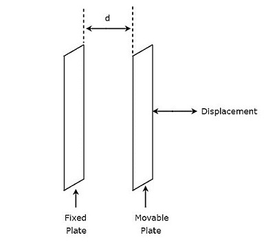
The capacitor, which is present in above circuit has two parallel plates. Among which, one plate is fixed and the other plate is a movable one. Due to this, the spacing between these two plates will also vary. the value of capacitance changes as the spacing between two plates of capacitor changes.

Therefore, we should connect the body whose displacement is to be measured to the movable plate of a capacitor. So, whenever the body moves in a straight line, the spacing between the two plates of capacitor varies. Due to this, the capacitance value changes.

Data Acquisition Systems

The systems, used for data acquisition are known as data acquisition systems. These data acquisition systems will perform the tasks such as conversion of data, storage of data, transmission of data and processing of data.

Data acquisition systems consider the following analog signals.

• Analog signals, which are obtained from the direct measurement of electrical quantities such as DC & AC voltages, DC & AC currents, resistance and etc.

• Analog signals, which are obtained from transducers such as LVDT, Thermocouple & etc.

Types of Data Acquisition Systems

Data acquisition systems can be classified into the following two types.

• Analog Data Acquisition Systems
• Digital Data Acquisition Systems

Now, let us discuss about these two types of data acquisition systems one by one.

Analog Data Acquisition Systems

The data acquisition systems, which can be operated with analog signals are known as analog data acquisition systems. Following are the blocks of analog data acquisition systems.

• Transducer − It converts physical quantities into electrical signals.

• Signal conditioner − It performs the functions like amplification and selection of desired portion of the signal.

• Display device − It displays the input signals for monitoring purpose.

• Graphic recording instruments − These can be used to make the record of input data permanently.

• Magnetic tape instrumentation − It is used for acquiring, storing & reproducing of input data.

Digital Data Acquisition Systems

The data acquisition systems, which can be operated with digital signals are known as digital data acquisition systems. So, they use digital components for storing or displaying the information.

Mainly, the following operations take place in digital data acquisition.

• Acquisition of analog signals
• Conversion of analog signals into digital signals or digital data
• Processing of digital signals or digital data

Following are the blocks of Digital data acquisition systems.

• Transducer − It converts physical quantities into electrical signals.

• Signal conditioner − It performs the functions like amplification and selection of desired portion of the signal.

• Multiplexer − connects one of the multiple inputs to output. So, it acts as parallel to serial converter.

• Analog to Digital Converter − It converts the analog input into its equivalent digital output.

• Display device − It displays the data in digital format.

• Digital Recorder − It is used to record the data in digital format.

Data acquisition systems are being used in various applications such as biomedical and aerospace. So, we can choose either analog data acquisition systems or digital data acquisition systems based on the requirement.