- Excel Power Pivot Tutorial
- Excel Power Pivot - Home
- Excel Power Pivot - Overview
- Excel Power Pivot - Installing
- Excel Power Pivot - Features
- Excel Power Pivot - Loading Data
- Excel Power Pivot - Data Model
- Power Pivot - Managing Data Model
- Excel Power Pivot Table - Creation
- Excel Power Pivot - Basics of DAX
- Power Pivot Table - Exploring Data
- Excel Power Pivot Table - Flattened
- Excel Power Pivot Charts - Creation
- Table & Chart Combinations
- Excel Power Pivot - Hierarchies
- Power Pivot - Aesthetic Reports
- Excel Power Pivot Useful Resources
- Excel Power Pivot - Quick Guide
- Excel Power Pivot - Resources
- Excel Power Pivot - Discussion
Excel Power PivotTable - Creation
Power PivotTable is based on the Power Pivot database, which is called the Data Model. You have already learnt the powerful features of the Data Model. The power of Power Pivot is in its ability to summarize data from the Data Model in the Power PivotTable. As you are aware, the Data Model can handle huge data spanning millions of rows and coming from diverse inputs. This enables Power PivotTable to summarize the data from anywhere in a matter of few minutes.
Power PivotTable resembles PivotTable in its layout, with the following differences −
PivotTable is based on Excel tables, whereas Power PivotTable is based on data tables that are part of Data Model.
PivotTable is based on a single Excel table or data range, whereas Power PivotTable can be based on multiple data tables, provided they are added to Data Model.
PivotTable is created from Excel window, whereas Power PivotTable is created from PowerPivot window.
Creating a Power PivotTable
Suppose you have two data tables − Salesperson and Sales in the Data Model. To create a PowerPivot Table from these two data tables, proceed as follows −
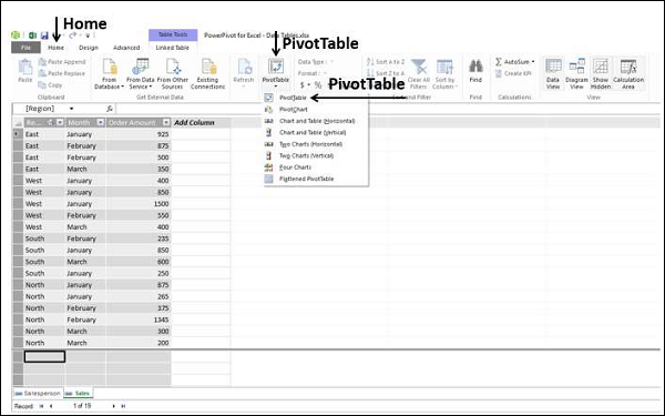
Click the Home tab on the Ribbon in PowerPivot window.
Click PivotTable on the Ribbon.
Select PivotTable from the dropdown list.
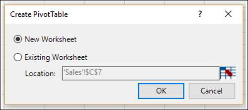
Create PivotTable dialog box appears. As you can observe, this is a simple dialog box, without any queries on data. This is because, Power PivotTable is always based on Data Model, i.e. the data tables with the relationships defined among them.
Select New Worksheet and click OK.
A new worksheet is created in Excel window and an empty PivotTable appears.
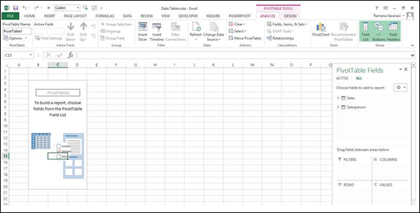
As you can observe, the layout of the Power PivotTable is similar to that of PivotTable. The PIVOTTABLE TOOLS appear on the Ribbon, with ANALYZE and DESIGN tabs, identical to PivotTable.
The PivotTable Fields List appears on the right side of the worksheet. Here, you will find some differences from PivotTable.
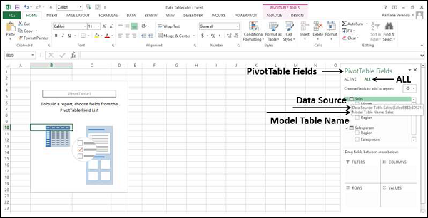
Power PivotTable Fields
The PivotTable Fields list has two tabs − ACTIVE and ALL that appear below the title and above the fields list. The ALL tab is highlighted.
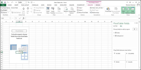
Note that the ALL tab displays all the data tables in the Data Model and ACTIVE tab displays all the data tables that are chosen for the Power PivotTable at hand. As the Power PivotTable is empty, it means that no data table is selected yet; hence by default, ALL tab is selected and the two tables that are currently in the Data Model are displayed. At this point, if you click the ACTIVE tab, the Fields list would be empty.
Click on the table names in the PivotTable Fields list under ALL. The corresponding fields with check boxes will appear.
Each table name will have the symbol
 on the left side.
If you place the cursor on this symbol, the Data Source and the Model Table Name of that data table will be displayed.
Drag Salesperson from Salesperson table to the ROWS area.
Click the ACTIVE tab.
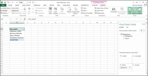
As you can observe, the field Salesperson appears in the PivotTable and the table Salesperson appears under the ACTIVE tab as expected.
Click the ALL tab.
Click on Month and Order Amount in the Sales table.
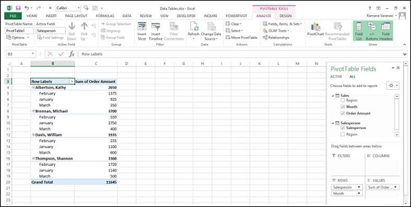
Again, click the ACTIVE tab. Both the tables − Sales and Salesperson appear under the ACTIVE tab.
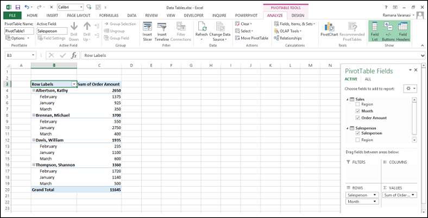
Drag Month to COLUMNS area.
Drag Region to FILTERS area.
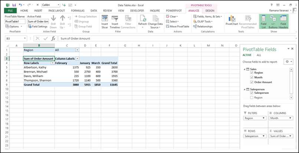
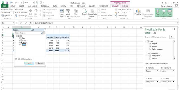
Click the arrow next to ALL in the Region filter box.
Click Select Multiple Items.
Select North and South and click OK.
Sort the column labels in the ascending order.
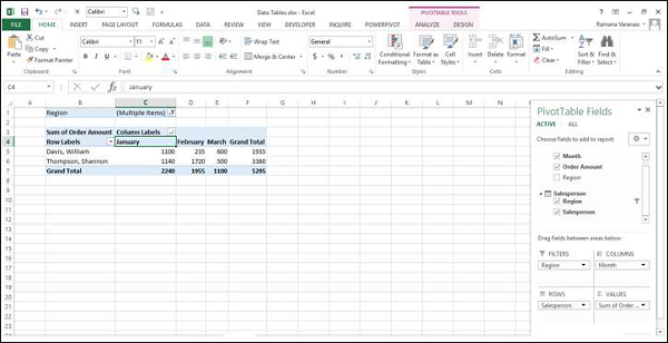
Power PivotTable can be modified dynamically explore and report data.