- Excel Power Pivot Tutorial
- Excel Power Pivot - Home
- Excel Power Pivot - Overview
- Excel Power Pivot - Installing
- Excel Power Pivot - Features
- Excel Power Pivot - Loading Data
- Excel Power Pivot - Data Model
- Power Pivot - Managing Data Model
- Excel Power Pivot Table - Creation
- Excel Power Pivot - Basics of DAX
- Power Pivot Table - Exploring Data
- Excel Power Pivot Table - Flattened
- Excel Power Pivot Charts - Creation
- Table & Chart Combinations
- Excel Power Pivot - Hierarchies
- Power Pivot - Aesthetic Reports
- Excel Power Pivot Useful Resources
- Excel Power Pivot - Quick Guide
- Excel Power Pivot - Resources
- Excel Power Pivot - Discussion
Excel Power Pivot - Basics of DAX
DAX (Data Analysis eXpression) language is the language of Power Pivot. DAX is used by Power Pivot for data modeling and it is convenient for you to use for self-service BI. DAX is based on data tables and columns in data tables. Note that it is not based on individual cells in the table as is the case with the formulas and functions in Excel.
You will learn the two simple calculations that exist in Data Model − Calculated Column and Calculated Field in this chapter.
Calculated Column
Calculated column is a column in the Data Model that is defined by a calculation and that extends the content of a data table. It can be visualized as a new column in an Excel table defined by a formula.
Extending the Data Model using Calculated Columns
Suppose you have sales data of products region-wise in data tables and also a Product Catalog in the Data Model.
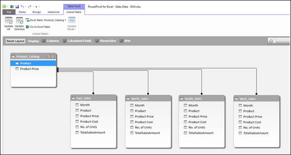
Create a Power PivotTable with this data.
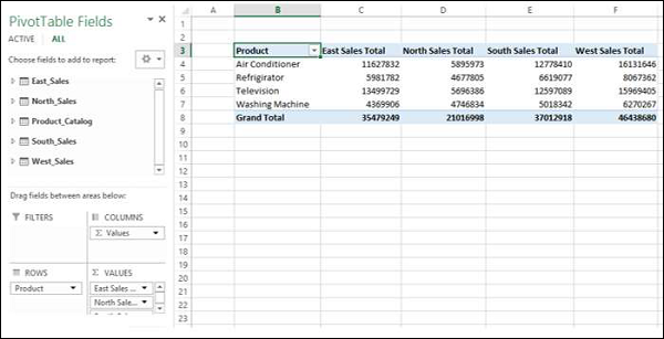
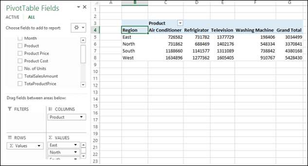
As you can observe, the Power PivotTable has summarized the sales data from all the regions. Suppose you want to know the gross profit made on each of the products. You know the price of each product, the cost at which it is sold and the number of units sold.
However, if you need to calculate the gross profit, you need to have two more columns in each of the data tables of the regions − Total Product Price and Gross Profit. This is because, PivotTable requires columns in data tables to summarize the results.
As you know, Total Product Price is Product Price * No. of Units and Gross Profit is Total Amount − Total Product Price.
You need to use DAX Expressions to add the Calculated Columns as follows −
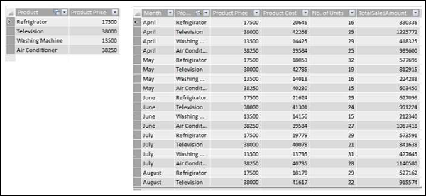
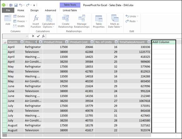
Click the East_Sales tab in Data View of the Power Pivot window to view the East_Sales Data Table.
Click the Design tab on the Ribbon.
Click Add.
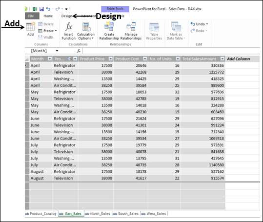
The column on the right side with the header − Add Column is highlighted.
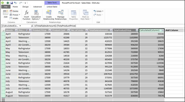
Type = [Product Price] * [No. of Units] in the formula bar and press Enter.
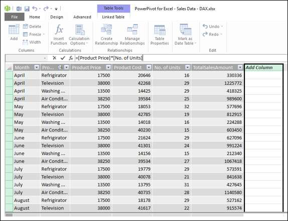
A new column with header CalculatedColumn1 is inserted with the values calculated by the formula you entered.
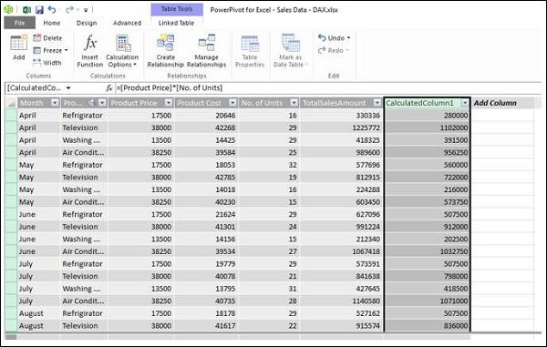
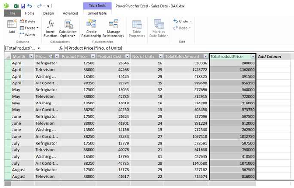
Double click the header of the new calculated column.
Rename the header as TotalProductPrice.
Add one more calculated column for Gross Profit as follows −
Click the Design tab on the Ribbon.
Click Add.
The column on the right side with the header − Add Column is highlighted.
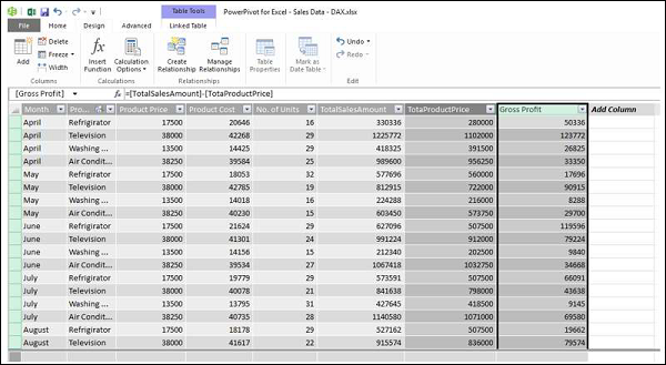
Type = [TotalSalesAmount] − [TotaProductPrice] in the formula bar.
Press Enter.
A new column with header CalculatedColumn1 is inserted with the values calculated by the formula you entered.
Double click the header of the new calculated column.
Rename the header as Gross Profit.
Add the Calculated Columns in the North_Sales data table in a similar way. Consolidating all the steps, proceed as follows −
Click the Design tab on the Ribbon.
Click Add. The column on the right side with the header − Add Column is highlighted.
Type = [Product Price] * [No. of Units] in the formula bar and press Enter.
A new column with header CalculatedColumn1 gets inserted with the values calculated by the formula you entered.
Double click the header of the new calculated column.
Rename the header as TotalProductPrice.
Click the Design tab on the Ribbon.
Click Add. The column on the right side with the header - Add Column is highlighted.
Type = [TotalSalesAmount] − [TotaProductPrice] in the formula bar and press Enter. A new column with header CalculatedColumn1 gets inserted with the values calculated by the formula you entered.
Double click the header of the new calculated column.
Rename the header as Gross Profit.
Repeat the above given steps for the South Sales data table and West Sales data table.
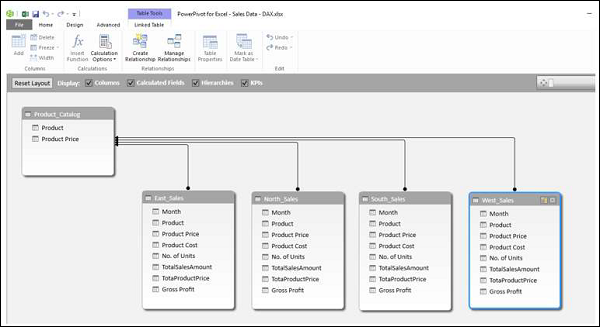
You have the necessary columns to summarize the Gross Profit. Now, create the Power PivotTable.
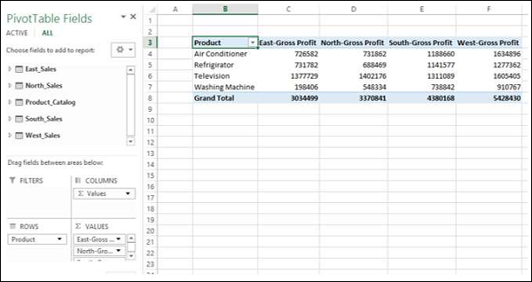
You are able to summarize the Gross Profit that became possible with the calculated columns in the Power Pivot and it all can be done just in a few steps that are error-free.
You can summarize it region wise for the products as given below also −
Calculated Field
Suppose you want to calculate the percentage of profit made by each region product-wise. You can do so by adding a calculated field to the Data Table.
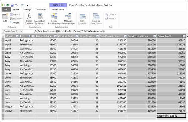
Click below the column Gross Profit in the East_Sales table in Power Pivot window.
Type EastProfit: = SUM ([Gross Profit]) / sum ([TotalSalesAmount]) in the formula bar.
Press Enter.
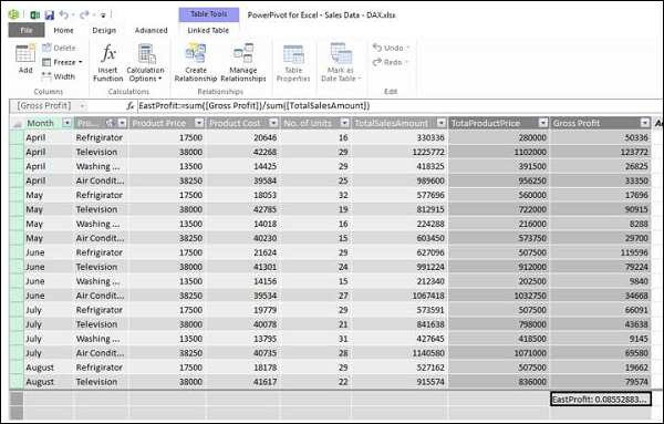
The calculated field EastProfit is inserted below the Gross Profit column.
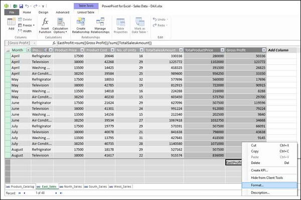
Right click the calculated field − EastProfit.
Select Format from the dropdown list.
The Formatting dialog box appears.
Select Number under Category.
In the Format box, select Percentage and click OK.
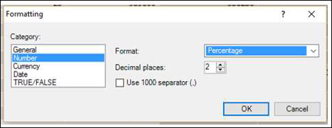
The calculated field EastProfit is formatted to percentage.
Repeat the steps to insert the following calculated fields −
NorthProfit in North_Sales data table.
SouthProfit in South_Sales data table.
WestProfit in West_Sales data table.
Note − You cannot define more than one calculated field with a given name.
Click on the Power PivotTable. You can see that the calculated fields appear in the tables.
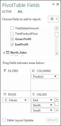
Select the fields − EastProfit, NorthProfit, SouthProfit and WestProfit from the tables in the PivotTable Fields list.
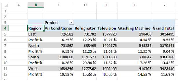
Arrange the fields such that the Gross Profit and Percentage Profit appear together. The Power PivotTable looks as follows −
Note − The Calculate Fields were called Measures in earlier versions of Excel.