- Excel Power Pivot Tutorial
- Excel Power Pivot - Home
- Excel Power Pivot - Overview
- Excel Power Pivot - Installing
- Excel Power Pivot - Features
- Excel Power Pivot - Loading Data
- Excel Power Pivot - Data Model
- Power Pivot - Managing Data Model
- Excel Power Pivot Table - Creation
- Excel Power Pivot - Basics of DAX
- Power Pivot Table - Exploring Data
- Excel Power Pivot Table - Flattened
- Excel Power Pivot Charts - Creation
- Table & Chart Combinations
- Excel Power Pivot - Hierarchies
- Power Pivot - Aesthetic Reports
- Excel Power Pivot Useful Resources
- Excel Power Pivot - Quick Guide
- Excel Power Pivot - Resources
- Excel Power Pivot - Discussion
Excel Power Pivot - Managing Data Model
The major use of Power Pivot is its ability to manage the data tables and the relationships among them, to facilitate analysis of the data from several tables. You can add an excel table to the Data Model while you are creating a PivotTable or directly from the PowerPivot Ribbon.
You can analyze data from across multiple tables only when relationships exist among them. With Power Pivot, you can create relationships from the Data View or Diagram View. Moreover, if you had chosen to add a table to the Power Pivot, you need to add a relationship as well.
Adding Excel Tables to Data Model with PivotTable
When you create a PivotTable in Excel, it is based only on a single table / range. In case you want to add more tables to the PivotTable, you can do so with the Data Model.
Suppose you have two worksheets in your workbook −
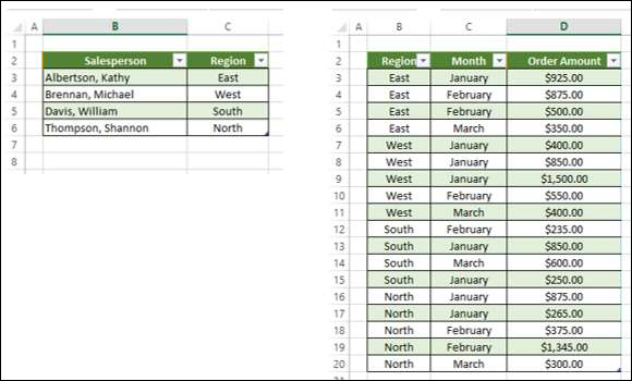
One containing the data of salespersons and the regions they represent, in a table- Salesperson.
Another containing the data of sales, region and month wise, in a table – Sales.

You can summarize the sales – salesperson-wise as given below.
Click the table – Sales.
Click the INSERT tab on the Ribbon.
Select PivotTable in the Tables group.
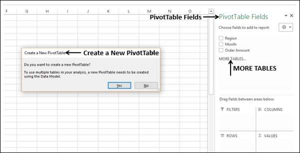
An empty PivotTable with the fields from the Sales table – Region, Month and Order Amount will be created. As you can observe, there is a MORE TABLES command below the PivotTable Fields list.
Click on MORE TABLES.
The Create a New PivotTable message box appears. The message displayed is- To use multiple tables in your analysis, a new PivotTable needs to be created using the Data Model. Click Yes
A New PivotTable will be created as shown below −
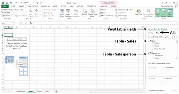
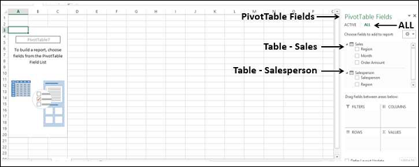
Under PivotTable Fields, you can observe that there are two tabs – ACTIVE and ALL.
Click the ALL tab.
Two tables- Sales and Salesperson, with the corresponding fields appear in the PivotTable Fields list.
Click the field Salesperson in the Salesperson table and drag it to ROWS area.
Click the field Month in the Sales table and drag it to ROWS area.
Click the field Order Amount in the Sales table and drag it to ∑ VALUES area.
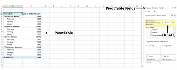
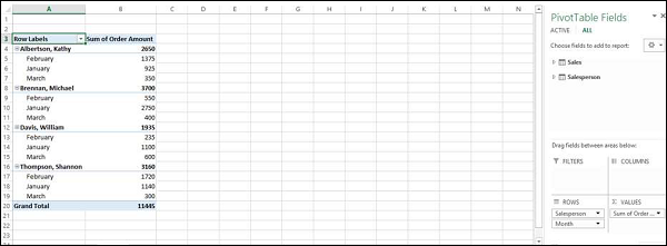
The PivotTable is created. A message appears in the PivotTable Fields – Relationships between tables may be needed.
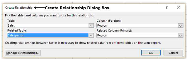
Click the CREATE button next to the message. The Create Relationship dialog box appears.
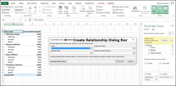
Under Table, select Sales.
Under Column (Foreign) box, select Region.
Under Related Table, select Salesperson.
Under Related Column (Primary) box, select Region.
Click OK.
Your PivotTable from the two tables on two worksheets is ready.
Further, as Excel stated while adding the second table to the PivotTable, the PivotTable got created with Data Model. To verify, do the following −
Click the POWERPIVOT tab on the Ribbon.
Click Manage in the Data Model group. The Data View of the Power Pivot appears.
You can observe that the two Excel tables that you used in creating the PivotTable are converted to data tables in the Data Model.
Adding Excel Tables from a Different Workbook to Data Model
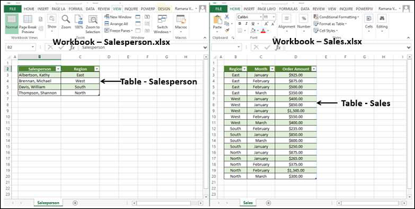
Suppose the two tables – Salesperson and Sales are in two different workbooks.
You can add the Excel table from a different workbook to the Data Model as follows −
Click the Sales table.
Click the INSERT tab.
Click PivotTable in the Tables group. The Create PivotTable dialog box appears.
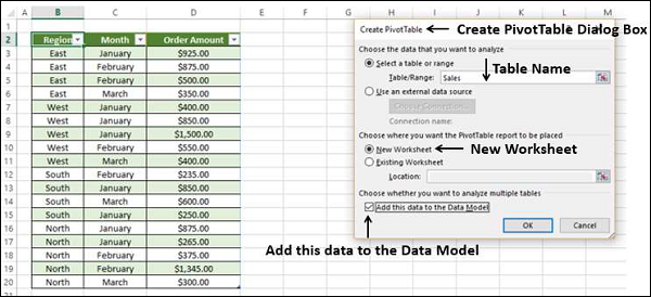
In the Table/Range box, type Sales.
Click on New Worksheet.
Check the box Add this data to the Data Model.
Click OK.
You will get an empty PivotTable on a new worksheet with only the fields corresponding to the Sales table.
You have added the Sales table data to the Data Model. Next, you have to get the Salesperson table data also into Data Model as follows −
Click on the worksheet containing Sales table.
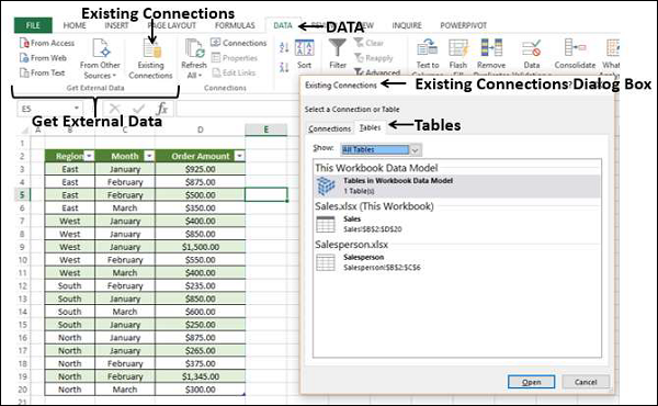
Click the DATA tab on the Ribbon.
Click Existing Connections in the Get External Data group. The Existing Connections dialog box appears.
Click on the Tables tab.
Under This Workbook Data Model, 1 table is displayed (This is the Sales table that you added earlier). You also find the two workbooks displaying the tables in them.
Click Salesperson under Salesperson.xlsx.
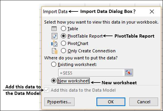
Click Open. The Import Data dialog box appears.
Click on PivotTable Report.
Click on New worksheet.
You can see that the box – Add this data to the Data Model is checked and inactive. Click OK.
The PivotTable will be created.
As you can observe the two tables are in the Data Model. You might have to create a relationship between the two tables as in the previous section.
Adding Excel Tables to Data Model from the PowerPivot Ribbon
Another way of adding Excel tables to Data Model is doing so from the PowerPivot Ribbon.
Suppose you have two worksheets in your workbook −
One containing the data of salespersons and the regions they represent, in a table – Salesperson.
Another containing the data of sales, region and month wise, in a table – Sales.
You can add these Excel tables to the Data Model first, before doing any analysis.
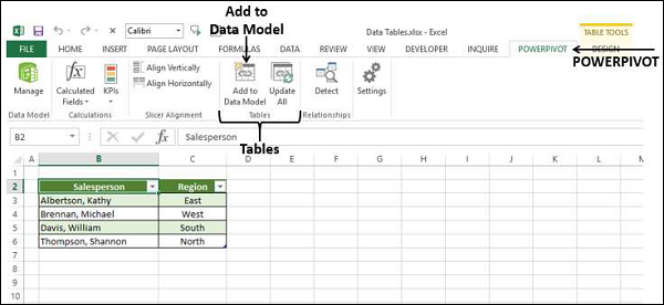
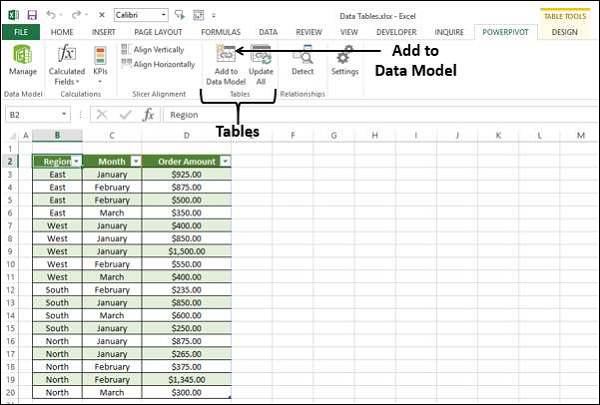
Click on the Excel table - Sales.
Click the POWERPIVOT tab on the Ribbon.
Click Add to Data Model in the Tables group.
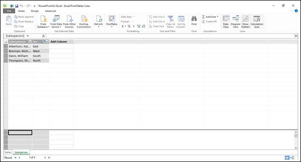
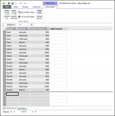
Power Pivot window appears, with the data table Salesperson added to it. Further a tab – Linked Table appears on the Ribbon in the Power Pivot window.
Click on the Linked Table tab on the Ribbon.
Click on Excel Table: Salesperson.
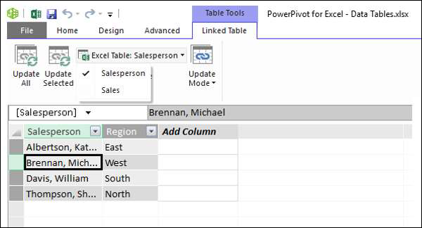
You can find that the names of the two tables present in your workbook are displayed and the name Salesperson is ticked. This means the data table Salesperson is linked to the Excel table Salesperson.
Click Go to Excel Table.
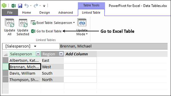
Excel window with worksheet containing Salesperson table appears.
Click the Sales worksheet tab.
Click the Sales table.
Click Add to Data Model in the Tables group on the Ribbon.
The Excel table Sales is also added to the Data Model.
If you want to do analysis based on these two tables, as you are aware, you need to create a relationship between the two data tables. In Power Pivot, you can do this in two ways −
From Data View
From Diagram View
Creating Relationships from Data View
As you know that in Data View, you can view the data tables with records as rows and fields as columns.
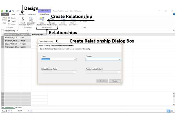
Click on the Design tab in the Power Pivot window.
Click on Create Relationship in the Relationships group. The Create Relationship dialog box appears.
Click on Sales in the Table box. This is the table from where the relationship starts. As you are aware, Column should be the field that is present in the related table Salesperson that contains unique values.
Click on Region in the Column box.
Click on Salesperson in the Related Linked Table box.
The Related Linked Column gets automatically populated with Region.
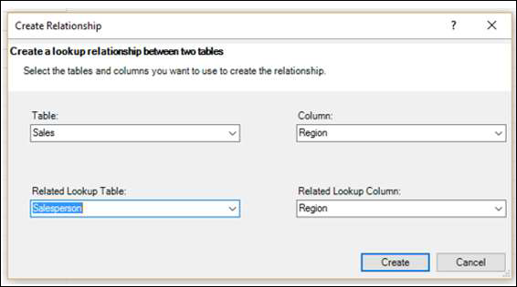
Click the Create button. The relationship is created.
Creating Relationships from Diagram View
Creating Relationships from Diagram View is relatively easier. Follow the given steps.
Click the Home tab in the Power Pivot window.
Click Diagram View in the View group.
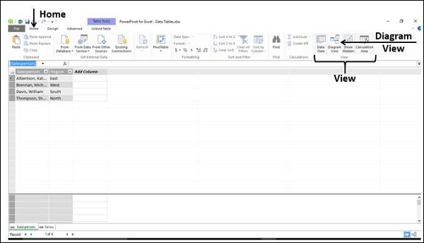
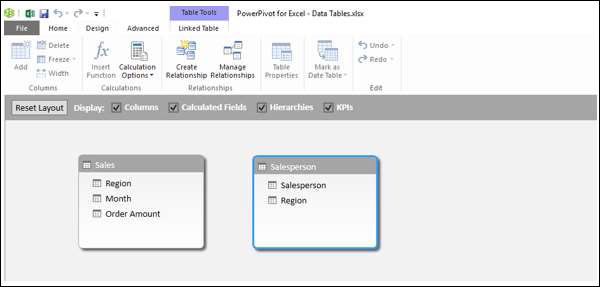
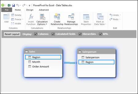
The Diagram View of the Data Model appears in the Power Pivot window.
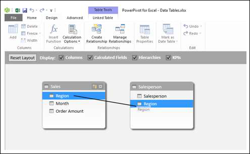
Click on Region in Sales table. Region in Sales table is highlighted.
Drag to Region in Salesperson table. Region in Salesperson table is also highlighted. A line appears in the direction you dragged.
A line appears from the table Sales to the table Salesperson indicating the relationship.
As you can see, a line appears from the Sales table to the Salesperson table, indicating the relationship and the direction.
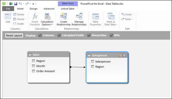
If you want to know the field that is a part of a relationship, click on the relationship line. The line and the field in both the tables are highlighted.
Managing Relationships
You can edit or delete an existing relationship in Data Model.
Click the Design tab in the Power Pivot window.
Click Manage Relationships in the Relationships group. The Manage Relationships dialog box appears.
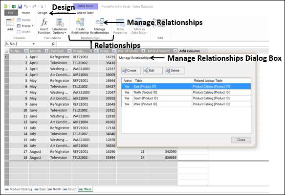
All the relationships that exist in the Data Model are displayed.
To edit a relationship
Click on a Relationship.
Click the Edit button. The Edit Relationship dialog box appears.
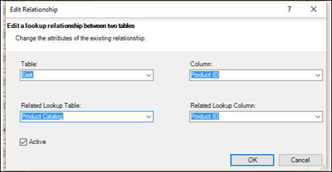
Make the required changes in the relationship.
Click OK. The changes get reflected in the relationship.
To delete a relationship
Click on a Relationship.
Click on the Delete button. A warning message appears showing how the tables that are affected by deleting the relationship would affect the reports.
Click OK if you are sure you want to delete. The selected relationship is deleted.
Refreshing Power Pivot Data
Suppose you modify the data in the Excel table. You can add / change / delete the data in the Excel table.
To refresh the PowerPivot data, do the following −
Click the Linked Table tab in the Power Pivot window.
Click Update All.
The data table is updated with the modifications made in the Excel table.
As you can observe, you cannot modify data in the data tables directly. Hence, it is better to maintain your data in Excel tables that are linked to the data tables when you add them to the Data Model. This facilitates updating the data in data tables as and when you update the data in Excel tables.
To Continue Learning Please Login