- TSSN - Home
- TSSN - Introduction
- TSSN - Switching Systems
- Elements of a Switching System
- TSSN - Strowger Switching System
- TSSN - Switching Mechanisms
- TSSN - Common Control
- TSSN - Touch-tone Dial Telephone
- TSSN - Crossbar Switching
- Crossbar Switch Configurations
- TSSN - Crosspoint Technology
- TSSN - Stored Program Control
- TSSN - Software Architecture
- TSSN - Switching Techniques
- TSSN - Time Division Switching
- TSSN - Telephone Networks
- TSSN - Signaling Techniques
- TSSN - ISDN
TSSN - Switching Techniques
In this chapter, we will discuss the switching techniques in Telecommunication Switching Systems and Networks.
In large networks, there may be more than one path for transmitting data from the sender to the receiver. Selecting a path that data must take out of the available options can be understood as Switching. The information may be switched while it travels between various communication channels.
There are three typical switching techniques available for digital traffic. They are −
- Circuit Switching
- Message Switching
- Packet Switching
Let us now see how these techniques work.
Circuit Switching
In Circuit switching, two nodes communicate with each other over a dedicated communication path. In this, a circuit is established to transfer the data. These circuits may be permanent or temporary. Applications that use circuit switching may have to go through three phases. The different phases are −
- Establishing a circuit
- Transferring the data
- Disconnecting the circuit
The following figure below shows the pattern of Circuit switching.
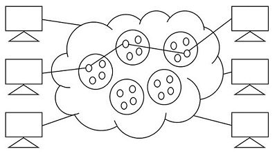
Circuit switching was designed for voice applications. Telephone is the best suitable example of circuit switching. Before a user can make a call, a virtual path between the called subscriber and the calling subscriber is established over the network.
The drawbacks of circuit switching are −
- The waiting time lasts long, and there is no data transfer.
- Each connection has a dedicated path, and this gets expensive.
- When connected systems do not use the channel, it is kept idle.
The circuit pattern is made once the connection is established, using the dedicated path which is intended for data transfer, in the circuit switching. The telephone system is a common example of Circuit Switching technique.
Message Switching
In message switching, the whole message is treated as a data unit. The data is transferred in its entire circuitry. A switch working on message switching, first receives the whole message and buffers it until there are resources available to transfer it to the next hop. If the next hop is not having enough resource to accommodate large size message, the message is stored and the switch waits.
The following figure shows the pattern of Message switching.
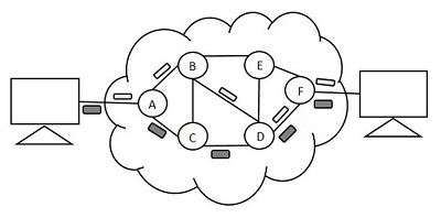
In this technique, the data is stored and forwarded. The technique is also called the Store-and-Forward technique. This technique was considered a substitute to circuit switching. But the transmission delay that followed the end to end delay of message transmission added to the propagation delay and slowed down the entire process.
Message switching has the following drawbacks −
Every switch in the transit path needs enough storage to accommodate the entire message.
Because of the waiting included until resources are available, message switching is very slow.
Message switching was not a solution for streaming media and real-time applications.
The data packets are accepted even when the network is busy; this slows down the delivery. Hence, this is not recommended for real time applications like voice and video.
Packet Switching
The packet switching technique is derived from message switching where the message is broken down into smaller chunks called Packets. The header of each packet contains the switching information which is then transmitted independently. The header contains details such as source, destination and intermediate node address information. The intermediate networking devices can store small size packets and dont take many resources either on the carrier path or in the internal memory of switches.
Individual routing of packets is done where a total set of packets need not be sent in the same route. As the data is split, bandwidth is reduced. This switching is used for performing data rate conversion.
The figure below shows the pattern of Packet switching.
The following figure shows the pattern of Packet switching.
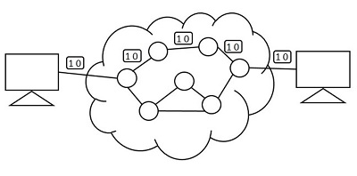
The line efficiency of packet switching can be enhanced by multiplexing the packets from multiple applications over the carrier. The internet which uses this packet switching enables the user to differentiate data streams based on priorities. Depending upon the priority list, these packets are forwarded after storing to provide quality of service.
The packet switching technique was proved to be an efficient technique and is being widely used in both voice and data transfer. The transmission resources are allocated using different techniques such as Statistical Multiplexing or Dynamic Bandwidth allocation.
Statistical Multiplexing
Statistical multiplexing is a communication link sharing technique, which is used in packet switching. The shared linking is variable in statistical multiplexing, whereas it is fixed in TDM or FDM. This is a strategic application for maximizing the utilization of bandwidth. This can increase the efficiency of network, as well.
By allocating the bandwidth for channels with valid data packets, statistical multiplexing technique combines the input traffic to maximize channel efficiency. Each stream is divided into packets, and delivered on a first-come, first-served basis. The increase in priority levels allow to allocate more bandwidth. The time slots are taken care not to be wasted in the statistical multiplexing whereas they are wasted in time division multiplexing.
Network Traffic
As the name implies, network traffic is simply the data that moves along the network in a given time. The data transmission is done in the form of packets, where the number of packets transmitted per unit time is considered as load. The controlling of this network traffic includes managing, prioritizing, controlling or reducing the network traffic. The amount and type of traffic on a network can also be measured with the help of a few techniques. The network traffic needs to be monitored as this helps in network security; high data rate might cause damage to the network.
A measure of the total work done by a resource or facility, over a period (usually 24 hours) is understood as Traffic Volume and is measured in Erlang-hours. The traffic volume is defined as the product of the average traffic intensity and the period of
$$Traffic \:\: volume = Traffic \: Intensity \times Time\: period$$
Congestion
Congestion in a network is said to have occurred when load on the network is greater than the capacity of the network. When the buffer size of the node exceeds the data received, then the traffic will be high. This further leads to congestion. The amount of data moved from a node to the other can be called as Throughput.
The following figure shows congestion.
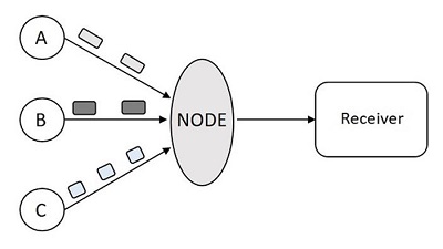
In the above figure, when the data packets arrive at Node from the senders A, B and C then the node cannot transmit the data to the receiver at a faster rate. There occurs a delay in transmission or may be data loss due to heavy congestion.
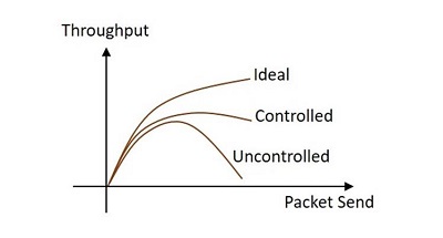
When too many packets arrive at the port in a packet switched network, then the performance degrades and such a situation is called Congestion. The data waits in the queue line for transmission. When the queue line is utilized more than 80%, then the queue line is said to be congested. The Congestion control techniques help in controlling the congestion. The following graph, drawn between throughput and packet send shows the difference between congestion controlled transmission and uncontrolled transmission.
The techniques used for congestion control are of two types open loop and closed loop. The loops differ by the protocols they issue.
Open Loop
The open loop congestion control mechanism produces protocols to avoid congestion. These protocols are sent to the source and the destination..
Closed Loop
The closed loop congestion control mechanism produces protocols that allow the system to enter the congested state and then detect and remove the congestion. The explicit and implicit feedback methods help in the running of the mechanism.
