- Home
- Basics
- Python Ecosystem
- Methods for Machine Learning
- Data Loading for ML Projects
- Understanding Data with Statistics
- Understanding Data with Visualization
- Preparing Data
- Data Feature Selection
- ML Algorithms - Classification
- Introduction
- Logistic Regression
- Support Vector Machine (SVM)
- Decision Tree
- Naïve Bayes
- Random Forest
- ML Algorithms - Regression
- Random Forest
- Linear Regression
- ML Algorithms - Clustering
- Overview
- K-means Algorithm
- Mean Shift Algorithm
- Hierarchical Clustering
- ML Algorithms - KNN Algorithm
- Finding Nearest Neighbors
- Performance Metrics
- Automatic Workflows
- Improving Performance of ML Models
- Improving Performance of ML Model (Contd…)
- ML With Python - Resources
- Machine Learning With Python - Quick Guide
- Machine Learning with Python - Resources
- Machine Learning With Python - Discussion
Machine Learning With Python - Quick Guide
Machine Learning with Python - Basics
We are living in the age of data that is enriched with better computational power and more storage resources,. This data or information is increasing day by day, but the real challenge is to make sense of all the data. Businesses & organizations are trying to deal with it by building intelligent systems using the concepts and methodologies from Data science, Data Mining and Machine learning. Among them, machine learning is the most exciting field of computer science. It would not be wrong if we call machine learning the application and science of algorithms that provides sense to the data.
What is Machine Learning?
Machine Learning (ML) is that field of computer science with the help of which computer systems can provide sense to data in much the same way as human beings do.
In simple words, ML is a type of artificial intelligence that extract patterns out of raw data by using an algorithm or method. The main focus of ML is to allow computer systems learn from experience without being explicitly programmed or human intervention.
Need for Machine Learning
Human beings, at this moment, are the most intelligent and advanced species on earth because they can think, evaluate and solve complex problems. On the other side, AI is still in its initial stage and havent surpassed human intelligence in many aspects. Then the question is that what is the need to make machine learn? The most suitable reason for doing this is, to make decisions, based on data, with efficiency and scale.
Lately, organizations are investing heavily in newer technologies like Artificial Intelligence, Machine Learning and Deep Learning to get the key information from data to perform several real-world tasks and solve problems. We can call it data-driven decisions taken by machines, particularly to automate the process. These data-driven decisions can be used, instead of using programing logic, in the problems that cannot be programmed inherently. The fact is that we cant do without human intelligence, but other aspect is that we all need to solve real-world problems with efficiency at a huge scale. That is why the need for machine learning arises.
Why & When to Make Machines Learn?
We have already discussed the need for machine learning, but another question arises that in what scenarios we must make the machine learn? There can be several circumstances where we need machines to take data-driven decisions with efficiency and at a huge scale. The followings are some of such circumstances where making machines learn would be more effective −
Lack of human expertise
The very first scenario in which we want a machine to learn and take data-driven decisions, can be the domain where there is a lack of human expertise. The examples can be navigations in unknown territories or spatial planets.
Dynamic scenarios
There are some scenarios which are dynamic in nature i.e. they keep changing over time. In case of these scenarios and behaviors, we want a machine to learn and take data-driven decisions. Some of the examples can be network connectivity and availability of infrastructure in an organization.
Difficulty in translating expertise into computational tasks
There can be various domains in which humans have their expertise,; however, they are unable to translate this expertise into computational tasks. In such circumstances we want machine learning. The examples can be the domains of speech recognition, cognitive tasks etc.
Machine Learning Model
Before discussing the machine learning model, we must need to understand the following formal definition of ML given by professor Mitchell −
A computer program is said to learn from experience E with respect to some class of tasks T and performance measure P, if its performance at tasks in T, as measured by P, improves with experience E.
The above definition is basically focusing on three parameters, also the main components of any learning algorithm, namely Task(T), Performance(P) and experience (E). In this context, we can simplify this definition as −
ML is a field of AI consisting of learning algorithms that −
Improve their performance (P)
At executing some task (T)
Over time with experience (E)
Based on the above, the following diagram represents a Machine Learning Model −

Let us discuss them more in detail now −
Task(T)
From the perspective of problem, we may define the task T as the real-world problem to be solved. The problem can be anything like finding best house price in a specific location or to find best marketing strategy etc. On the other hand, if we talk about machine learning, the definition of task is different because it is difficult to solve ML based tasks by conventional programming approach.
A task T is said to be a ML based task when it is based on the process and the system must follow for operating on data points. The examples of ML based tasks are Classification, Regression, Structured annotation, Clustering, Transcription etc.
Experience (E)
As name suggests, it is the knowledge gained from data points provided to the algorithm or model. Once provided with the dataset, the model will run iteratively and will learn some inherent pattern. The learning thus acquired is called experience(E). Making an analogy with human learning, we can think of this situation as in which a human being is learning or gaining some experience from various attributes like situation, relationships etc. Supervised, unsupervised and reinforcement learning are some ways to learn or gain experience. The experience gained by out ML model or algorithm will be used to solve the task T.
Performance (P)
An ML algorithm is supposed to perform task and gain experience with the passage of time. The measure which tells whether ML algorithm is performing as per expectation or not is its performance (P). P is basically a quantitative metric that tells how a model is performing the task, T, using its experience, E. There are many metrics that help to understand the ML performance, such as accuracy score, F1 score, confusion matrix, precision, recall, sensitivity etc.
Challenges in Machines Learning
While Machine Learning is rapidly evolving, making significant strides with cybersecurity and autonomous cars, this segment of AI as whole still has a long way to go. The reason behind is that ML has not been able to overcome number of challenges. The challenges that ML is facing currently are −
Quality of data − Having good-quality data for ML algorithms is one of the biggest challenges. Use of low-quality data leads to the problems related to data preprocessing and feature extraction.
Time-Consuming task − Another challenge faced by ML models is the consumption of time especially for data acquisition, feature extraction and retrieval.
Lack of specialist persons − As ML technology is still in its infancy stage, availability of expert resources is a tough job.
No clear objective for formulating business problems − Having no clear objective and well-defined goal for business problems is another key challenge for ML because this technology is not that mature yet.
Issue of overfitting & underfitting − If the model is overfitting or underfitting, it cannot be represented well for the problem.
Curse of dimensionality − Another challenge ML model faces is too many features of data points. This can be a real hindrance.
Difficulty in deployment − Complexity of the ML model makes it quite difficult to be deployed in real life.
Applications of Machines Learning
Machine Learning is the most rapidly growing technology and according to researchers we are in the golden year of AI and ML. It is used to solve many real-world complex problems which cannot be solved with traditional approach. Following are some real-world applications of ML −
Emotion analysis
Sentiment analysis
Error detection and prevention
Weather forecasting and prediction
Stock market analysis and forecasting
Speech synthesis
Speech recognition
Customer segmentation
Object recognition
Fraud detection
Fraud prevention
Recommendation of products to customer in online shopping.
Machine Learning with Python - Ecosystem
An Introduction to Python
Python is a popular object-oriented programing language having the capabilities of high-level programming language. Its easy to learn syntax and portability capability makes it popular these days. The followings facts gives us the introduction to Python −
Python was developed by Guido van Rossum at Stichting Mathematisch Centrum in the Netherlands.
It was written as the successor of programming language named ABC.
Its first version was released in 1991.
The name Python was picked by Guido van Rossum from a TV show named Monty Pythons Flying Circus.
It is an open source programming language which means that we can freely download it and use it to develop programs. It can be downloaded from www.python.org.
Python programming language is having the features of Java and C both. It is having the elegant C code and on the other hand, it is having classes and objects like Java for object-oriented programming.
It is an interpreted language, which means the source code of Python program would be first converted into bytecode and then executed by Python virtual machine.
Strengths and Weaknesses of Python
Every programming language has some strengths as well as weaknesses, so does Python too.
Strengths
According to studies and surveys, Python is the fifth most important language as well as the most popular language for machine learning and data science. It is because of the following strengths that Python has −
Easy to learn and understand − The syntax of Python is simpler; hence it is relatively easy, even for beginners also, to learn and understand the language.
Multi-purpose language − Python is a multi-purpose programming language because it supports structured programming, object-oriented programming as well as functional programming.
Huge number of modules − Python has huge number of modules for covering every aspect of programming. These modules are easily available for use hence making Python an extensible language.
Support of open source community − As being open source programming language, Python is supported by a very large developer community. Due to this, the bugs are easily fixed by the Python community. This characteristic makes Python very robust and adaptive.
Scalability − Python is a scalable programming language because it provides an improved structure for supporting large programs than shell-scripts.
Weakness
Although Python is a popular and powerful programming language, it has its own weakness of slow execution speed.
The execution speed of Python is slow as compared to compiled languages because Python is an interpreted language. This can be the major area of improvement for Python community.
Installing Python
For working in Python, we must first have to install it. You can perform the installation of Python in any of the following two ways −
Installing Python individually
Using Pre-packaged Python distribution − Anaconda
Let us discuss these each in detail.
Installing Python Individually
If you want to install Python on your computer, then then you need to download only the binary code applicable for your platform. Python distribution is available for Windows, Linux and Mac platforms.
The following is a quick overview of installing Python on the above-mentioned platforms −
On Unix and Linux platform
With the help of following steps, we can install Python on Unix and Linux platform −
First, go to https://www.python.org/downloads/.
Next, click on the link to download zipped source code available for Unix/Linux.
Now, Download and extract files.
Next, we can edit the Modules/Setup file if we want to customize some options.
Next, write the command run ./configure script
make
make install
On Windows platform
With the help of following steps, we can install Python on Windows platform −
First, go to https://www.python.org/downloads/.
Next, click on the link for Windows installer python-XYZ.msi file. Here XYZ is the version we wish to install.
Now, we must run the file that is downloaded. It will take us to the Python install wizard, which is easy to use. Now, accept the default settings and wait until the install is finished.
On Macintosh platform
For Mac OS X, Homebrew, a great and easy to use package installer is recommended to install Python 3. In case if you don't have Homebrew, you can install it with the help of following command −
$ ruby -e "$(curl -fsSL
https://raw.githubusercontent.com/Homebrew/install/master/install)"
It can be updated with the command below −
$ brew update
Now, to install Python3 on your system, we need to run the following command −
$ brew install python3
Using Pre-packaged Python Distribution: Anaconda
Anaconda is a packaged compilation of Python which have all the libraries widely used in Data science. We can follow the following steps to setup Python environment using Anaconda −
Step1 − First, we need to download the required installation package from Anaconda distribution. The link for the same is https://www.anaconda.com/distribution/. You can choose from Windows, Mac and Linux OS as per your requirement.
Step2 − Next, select the Python version you want to install on your machine. The latest Python version is 3.7. There you will get the options for 64-bit and 32-bit Graphical installer both.
Step3 − After selecting the OS and Python version, it will download the Anaconda installer on your computer. Now, double click the file and the installer will install Anaconda package.
Step4 − For checking whether it is installed or not, open a command prompt and type Python as follows −

You can also check this in detailed video lecture athttps://www.tutorialspoint.com/python_essentials_online_training/getting_started_with_anaconda.asp.
Why Python for Data Science?
Python is the fifth most important language as well as most popular language for Machine learning and data science. The following are the features of Python that makes it the preferred choice of language for data science −
Extensive set of packages
Python has an extensive and powerful set of packages which are ready to be used in various domains. It also has packages like numpy, scipy, pandas, scikit-learn etc. which are required for machine learning and data science.
Easy prototyping
Another important feature of Python that makes it the choice of language for data science is the easy and fast prototyping. This feature is useful for developing new algorithm.
Collaboration feature
The field of data science basically needs good collaboration and Python provides many useful tools that make this extremely.
One language for many domains
A typical data science project includes various domains like data extraction, data manipulation, data analysis, feature extraction, modelling, evaluation, deployment and updating the solution. As Python is a multi-purpose language, it allows the data scientist to address all these domains from a common platform.
Components of Python ML Ecosystem
In this section, let us discuss some core Data Science libraries that form the components of Python Machine learning ecosystem. These useful components make Python an important language for Data Science. Though there are many such components, let us discuss some of the importance components of Python ecosystem here −
Jupyter Notebook
Jupyter notebooks basically provides an interactive computational environment for developing Python based Data Science applications. They are formerly known as ipython notebooks. The following are some of the features of Jupyter notebooks that makes it one of the best components of Python ML ecosystem −
Jupyter notebooks can illustrate the analysis process step by step by arranging the stuff like code, images, text, output etc. in a step by step manner.
It helps a data scientist to document the thought process while developing the analysis process.
One can also capture the result as the part of the notebook.
With the help of jupyter notebooks, we can share our work with a peer also.
Installation and Execution
If you are using Anaconda distribution, then you need not install jupyter notebook separately as it is already installed with it. You just need to go to Anaconda Prompt and type the following command −
C:\>jupyter notebook
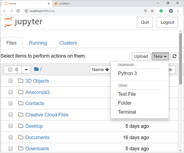
After pressing enter, it will start a notebook server at localhost:8888 of your computer. It is shown in the following screen shot −

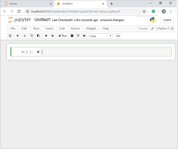
Now, after clicking the New tab, you will get a list of options. Select Python 3 and it will take you to the new notebook for start working in it. You will get a glimpse of it in the following screenshots −
On the other hand, if you are using standard Python distribution then jupyter notebook can be installed using popular python package installer, pip.
pip install jupyter
Types of Cells in Jupyter Notebook
The following are the three types of cells in a jupyter notebook −
Code cells − As the name suggests, we can use these cells to write code. After writing the code/content, it will send it to the kernel that is associated with the notebook.
Markdown cells − We can use these cells for notating the computation process. They can contain the stuff like text, images, Latex equations, HTML tags etc.
Raw cells − The text written in them is displayed as it is. These cells are basically used to add the text that we do not wish to be converted by the automatic conversion mechanism of jupyter notebook.
For more detailed study of jupyter notebook, you can go to the linkhttps://www.tutorialspoint.com/jupyter/index.htm.
NumPy
It is another useful component that makes Python as one of the favorite languages for Data Science. It basically stands for Numerical Python and consists of multidimensional array objects. By using NumPy, we can perform the following important operations −
Mathematical and logical operations on arrays.
Fourier transformation
Operations associated with linear algebra.
We can also see NumPy as the replacement of MatLab because NumPy is mostly used along with Scipy (Scientific Python) and Mat-plotlib (plotting library).
Installation and Execution
If you are using Anaconda distribution, then no need to install NumPy separately as it is already installed with it. You just need to import the package into your Python script with the help of following −
import numpy as np
On the other hand, if you are using standard Python distribution then NumPy can be installed using popular python package installer, pip.
pip install NumPy
For more detailed study of NumPy, you can go to the link https://www.tutorialspoint.com/numpy/index.htm.
Pandas
It is another useful Python library that makes Python one of the favorite languages for Data Science. Pandas is basically used for data manipulation, wrangling and analysis. It was developed by Wes McKinney in 2008. With the help of Pandas, in data processing we can accomplish the following five steps −
Load
Prepare
Manipulate
Model
Analyze
Data representation in Pandas
The entire representation of data in Pandas is done with the help of following three data structures −
Series − It is basically a one-dimensional ndarray with an axis label which means it is like a simple array with homogeneous data. For example, the following series is a collection of integers 1,5,10,15,24,25
| 1 | 5 | 10 | 15 | 24 | 25 | 28 | 36 | 40 | 89 |
Data frame − It is the most useful data structure and used for almost all kind of data representation and manipulation in pandas. It is basically a two-dimensional data structure which can contain heterogeneous data. Generally, tabular data is represented by using data frames. For example, the following table shows the data of students having their names and roll numbers, age and gender −
Name |
Roll number |
Age |
Gender |
|---|---|---|---|
Aarav |
1 |
15 |
Male |
Harshit |
2 |
14 |
Male |
Kanika |
3 |
16 |
Female |
Mayank |
4 |
15 |
Male |
Panel − It is a 3-dimensional data structure containing heterogeneous data. It is very difficult to represent the panel in graphical representation, but it can be illustrated as a container of DataFrame.
The following table gives us the dimension and description about above mentioned data structures used in Pandas −
Data Structure |
Dimension |
Description |
|---|---|---|
Series |
1-D |
Size immutable, 1-D homogeneous data |
DataFrames |
2-D |
Size Mutable, Heterogeneous data in tabular form |
Panel |
3-D |
Size-mutable array, container of DataFrame. |
We can understand these data structures as the higher dimensional data structure is the container of lower dimensional data structure.
Installation and Execution
If you are using Anaconda distribution, then no need to install Pandas separately as it is already installed with it. You just need to import the package into your Python script with the help of following −
import pandas as pd
On the other hand, if you are using standard Python distribution then Pandas can be installed using popular python package installer, pip.
pip install Pandas
After installing Pandas, you can import it into your Python script as did above.
Example
The following is an example of creating a series from ndarray by using Pandas −
In [1]: import pandas as pd

In [2]: import numpy as np

In [3]: data = np.array(['g','a','u','r','a','v'])

In [4]: s = pd.Series(data)

In [5]: print (s)

0 g
1 a
2 u
3 r
4 a
5 v

dtype: object
For more detailed study of Pandas you can go to the link https://www.tutorialspoint.com/python_pandas/index.htm.
Scikit-learn
Another useful and most important python library for Data Science and machine learning in Python is Scikit-learn. The following are some features of Scikit-learn that makes it so useful −
It is built on NumPy, SciPy, and Matplotlib.
It is an open source and can be reused under BSD license.
It is accessible to everybody and can be reused in various contexts.
Wide range of machine learning algorithms covering major areas of ML like classification, clustering, regression, dimensionality reduction, model selection etc. can be implemented with the help of it.
Installation and Execution
If you are using Anaconda distribution, then no need to install Scikit-learn separately as it is already installed with it. You just need to use the package into your Python script. For example, with following line of script we are importing dataset of breast cancer patients from Scikit-learn −
from sklearn.datasets import load_breast_cancer
On the other hand, if you are using standard Python distribution and having NumPy and SciPy then Scikit-learn can be installed using popular python package installer, pip.
pip install -U scikit-learn
After installing Scikit-learn, you can use it into your Python script as you have done above.
Machine Learning with Python - Methods
There are various ML algorithms, techniques and methods that can be used to build models for solving real-life problems by using data. In this chapter, we are going to discuss such different kinds of methods.
Different Types of Methods
The following are various ML methods based on some broad categories −
Based on human supervision
In the learning process, some of the methods that are based on human supervision are as follows −
Supervised Learning
Supervised learning algorithms or methods are the most commonly used ML algorithms. This method or learning algorithm take the data sample i.e. the training data and its associated output i.e. labels or responses with each data samples during the training process.
The main objective of supervised learning algorithms is to learn an association between input data samples and corresponding outputs after performing multiple training data instances.
For example, we have
x: Input variables and
Y: Output variable
Now, apply an algorithm to learn the mapping function from the input to output as follows −
Y=f(x)
Now, the main objective would be to approximate the mapping function so well that even when we have new input data (x), we can easily predict the output variable (Y) for that new input data.
It is called supervised because the whole process of learning can be thought as it is being supervised by a teacher or supervisor. Examples of supervised machine learning algorithms includes Decision tree, Random Forest, KNN, Logistic Regression etc.
Based on the ML tasks, supervised learning algorithms can be divided into following two broad classes −
Classification
Regression
Classification
The key objective of classification-based tasks is to predict categorial output labels or responses for the given input data. The output will be based on what the model has learned in training phase. As we know that the categorial output responses means unordered and discrete values, hence each output response will belong to a specific class or category. We will discuss Classification and associated algorithms in detail in the upcoming chapters also.
Regression
The key objective of regression-based tasks is to predict output labels or responses which are continues numeric values, for the given input data. The output will be based on what the model has learned in its training phase. Basically, regression models use the input data features (independent variables) and their corresponding continuous numeric output values (dependent or outcome variables) to learn specific association between inputs and corresponding outputs. We will discuss regression and associated algorithms in detail in further chapters also.
Unsupervised Learning
As the name suggests, it is opposite to supervised ML methods or algorithms which means in unsupervised machine learning algorithms we do not have any supervisor to provide any sort of guidance. Unsupervised learning algorithms are handy in the scenario in which we do not have the liberty, like in supervised learning algorithms, of having pre-labeled training data and we want to extract useful pattern from input data.
For example, it can be understood as follows −
Suppose we have −
x: Input variables, then there would be no corresponding output variable and the algorithms need to discover the interesting pattern in data for learning.
Examples of unsupervised machine learning algorithms includes K-means clustering, K-nearest neighbors etc.
Based on the ML tasks, unsupervised learning algorithms can be divided into following broad classes −
Clustering
Association
Dimensionality Reduction
Clustering
Clustering methods are one of the most useful unsupervised ML methods. These algorithms used to find similarity as well as relationship patterns among data samples and then cluster those samples into groups having similarity based on features. The real-world example of clustering is to group the customers by their purchasing behavior.
Association
Another useful unsupervised ML method is Association which is used to analyze large dataset to find patterns which further represents the interesting relationships between various items. It is also termed as Association Rule Mining or Market basket analysis which is mainly used to analyze customer shopping patterns.
Dimensionality Reduction
This unsupervised ML method is used to reduce the number of feature variables for each data sample by selecting set of principal or representative features. A question arises here is that why we need to reduce the dimensionality? The reason behind is the problem of feature space complexity which arises when we start analyzing and extracting millions of features from data samples. This problem generally refers to curse of dimensionality. PCA (Principal Component Analysis), K-nearest neighbors and discriminant analysis are some of the popular algorithms for this purpose.
Anomaly Detection
This unsupervised ML method is used to find out the occurrences of rare events or observations that generally do not occur. By using the learned knowledge, anomaly detection methods would be able to differentiate between anomalous or a normal data point. Some of the unsupervised algorithms like clustering, KNN can detect anomalies based on the data and its features.
Semi-supervised Learning
Such kind of algorithms or methods are neither fully supervised nor fully unsupervised. They basically fall between the two i.e. supervised and unsupervised learning methods. These kinds of algorithms generally use small supervised learning component i.e. small amount of pre-labeled annotated data and large unsupervised learning component i.e. lots of unlabeled data for training. We can follow any of the following approaches for implementing semi-supervised learning methods −
The first and simple approach is to build the supervised model based on small amount of labeled and annotated data and then build the unsupervised model by applying the same to the large amounts of unlabeled data to get more labeled samples. Now, train the model on them and repeat the process.
- ,p>The second approach needs some extra efforts. In this approach, we can first use the unsupervised methods to cluster similar data samples, annotate these groups and then use a combination of this information to train the model.
Reinforcement Learning
These methods are different from previously studied methods and very rarely used also. In this kind of learning algorithms, there would be an agent that we want to train over a period of time so that it can interact with a specific environment. The agent will follow a set of strategies for interacting with the environment and then after observing the environment it will take actions regards the current state of the environment. The following are the main steps of reinforcement learning methods −
Step1 − First, we need to prepare an agent with some initial set of strategies.
Step2 − Then observe the environment and its current state.
Step3 − Next, select the optimal policy regards the current state of the environment and perform important action.
Step4 − Now, the agent can get corresponding reward or penalty as per accordance with the action taken by it in previous step.
Step5 − Now, we can update the strategies if it is required so.
Step6 − At last, repeat steps 2-5 until the agent got to learn and adopt the optimal policies.
Tasks Suited for Machine Learning
The following diagram shows what type of task is appropriate for various ML problems −

Based on learning ability
In the learning process, the following are some methods that are based on learning ability −
Batch Learning
In many cases, we have end-to-end Machine Learning systems in which we need to train the model in one go by using whole available training data. Such kind of learning method or algorithm is called Batch or Offline learning. It is called Batch or Offline learning because it is a one-time procedure and the model will be trained with data in one single batch. The following are the main steps of Batch learning methods −
Step1 − First, we need to collect all the training data for start training the model.
Step2 − Now, start the training of model by providing whole training data in one go.
Step3 − Next, stop learning/training process once you got satisfactory results/performance.
Step4 − Finally, deploy this trained model into production. Here, it will predict the output for new data sample.
Online Learning
It is completely opposite to the batch or offline learning methods. In these learning methods, the training data is supplied in multiple incremental batches, called mini-batches, to the algorithm. Followings are the main steps of Online learning methods −
Step1 − First, we need to collect all the training data for starting training of the model.
Step2 − Now, start the training of model by providing a mini-batch of training data to the algorithm.
Step3 − Next, we need to provide the mini-batches of training data in multiple increments to the algorithm.
Step4 − As it will not stop like batch learning hence after providing whole training data in mini-batches, provide new data samples also to it.
Step5 − Finally, it will keep learning over a period of time based on the new data samples.
Based on Generalization Approach
In the learning process, followings are some methods that are based on generalization approaches −
Instance based Learning
Instance based learning method is one of the useful methods that build the ML models by doing generalization based on the input data. It is opposite to the previously studied learning methods in the way that this kind of learning involves ML systems as well as methods that uses the raw data points themselves to draw the outcomes for newer data samples without building an explicit model on training data.
In simple words, instance-based learning basically starts working by looking at the input data points and then using a similarity metric, it will generalize and predict the new data points.
Model based Learning
In Model based learning methods, an iterative process takes place on the ML models that are built based on various model parameters, called hyperparameters and in which input data is used to extract the features. In this learning, hyperparameters are optimized based on various model validation techniques. That is why we can say that Model based learning methods uses more traditional ML approach towards generalization.
Data Loading for ML Projects
Suppose if you want to start a ML project then what is the first and most important thing you would require? It is the data that we need to load for starting any of the ML project. With respect to data, the most common format of data for ML projects is CSV (comma-separated values).
Basically, CSV is a simple file format which is used to store tabular data (number and text) such as a spreadsheet in plain text. In Python, we can load CSV data into with different ways but before loading CSV data we must have to take care about some considerations.
Consideration While Loading CSV data
CSV data format is the most common format for ML data, but we need to take care about following major considerations while loading the same into our ML projects −
File Header
In CSV data files, the header contains the information for each field. We must use the same delimiter for the header file and for data file because it is the header file that specifies how should data fields be interpreted.
The following are the two cases related to CSV file header which must be considered −
Case-I: When Data file is having a file header − It will automatically assign the names to each column of data if data file is having a file header.
Case-II: When Data file is not having a file header − We need to assign the names to each column of data manually if data file is not having a file header.
In both the cases, we must need to specify explicitly weather our CSV file contains header or not.
Comments
Comments in any data file are having their significance. In CSV data file, comments are indicated by a hash (#) at the start of the line. We need to consider comments while loading CSV data into ML projects because if we are having comments in the file then we may need to indicate, depends upon the method we choose for loading, whether to expect those comments or not.
Delimiter
In CSV data files, comma (,) character is the standard delimiter. The role of delimiter is to separate the values in the fields. It is important to consider the role of delimiter while uploading the CSV file into ML projects because we can also use a different delimiter such as a tab or white space. But in the case of using a different delimiter than standard one, we must have to specify it explicitly.
Quotes
In CSV data files, double quotation ( ) mark is the default quote character. It is important to consider the role of quotes while uploading the CSV file into ML projects because we can also use other quote character than double quotation mark. But in case of using a different quote character than standard one, we must have to specify it explicitly.
Methods to Load CSV Data File
While working with ML projects, the most crucial task is to load the data properly into it. The most common data format for ML projects is CSV and it comes in various flavors and varying difficulties to parse. In this section, we are going to discuss about three common approaches in Python to load CSV data file −
Load CSV with Python Standard Library
The first and most used approach to load CSV data file is the use of Python standard library which provides us a variety of built-in modules namely csv module and the reader()function. The following is an example of loading CSV data file with the help of it −
Example
In this example, we are using the iris flower data set which can be downloaded into our local directory. After loading the data file, we can convert it into NumPy array and use it for ML projects. Following is the Python script for loading CSV data file −
First, we need to import the csv module provided by Python standard library as follows −
import csv
Next, we need to import Numpy module for converting the loaded data into NumPy array.
import numpy as np
Now, provide the full path of the file, stored on our local directory, having the CSV data file −
path = r"c:\iris.csv"
Next, use the csv.reader()function to read data from CSV file −
with open(path,'r') as f:
   reader = csv.reader(f,delimiter = ',')
   headers = next(reader)
   data = list(reader)
   data = np.array(data).astype(float)
We can print the names of the headers with the following line of script −
print(headers)
The following line of script will print the shape of the data i.e. number of rows & columns in the file −
print(data.shape)
Next script line will give the first three line of data file −
print(data[:3])
Output
['sepal_length', 'sepal_width', 'petal_length', 'petal_width']
(150, 4)
[  [5.1 3.5 1.4 0.2]
   [4.9 3. 1.4 0.2]
   [4.7 3.2 1.3 0.2]]
Load CSV with NumPy
Another approach to load CSV data file is NumPy and numpy.loadtxt() function. The following is an example of loading CSV data file with the help of it −
Example
In this example, we are using the Pima Indians Dataset having the data of diabetic patients. This dataset is a numeric dataset with no header. It can also be downloaded into our local directory. After loading the data file, we can convert it into NumPy array and use it for ML projects. The following is the Python script for loading CSV data file −
from numpy import loadtxt
path = r"C:\pima-indians-diabetes.csv"
datapath= open(path, 'r')
data = loadtxt(datapath, delimiter=",")
print(data.shape)
print(data[:3])
Output
(768, 9)
[  [ 6. 148. 72. 35. 0. 33.6 0.627 50. 1.]
   [ 1. 85. 66. 29. 0. 26.6 0.351 31. 0.]
   [ 8. 183. 64. 0. 0. 23.3 0.672 32. 1.]]
Load CSV with Pandas
Another approach to load CSV data file is by Pandas and pandas.read_csv()function. This is the very flexible function that returns a pandas.DataFrame which can be used immediately for plotting. The following is an example of loading CSV data file with the help of it −
Example
Here, we will be implementing two Python scripts, first is with Iris data set having headers and another is by using the Pima Indians Dataset which is a numeric dataset with no header. Both the datasets can be downloaded into local directory.
Script-1
The following is the Python script for loading CSV data file using Pandas on Iris Data set −
from pandas import read_csv
path = r"C:\iris.csv"
data = read_csv(path)
print(data.shape)
print(data[:3])

Output:

(150, 4)
   sepal_length   sepal_width  petal_length   petal_width
0         5.1     3.5          1.4            0.2
1         4.9     3.0          1.4            0.2
2         4.7     3.2          1.3            0.2
Script-2
The following is the Python script for loading CSV data file, along with providing the headers names too, using Pandas on Pima Indians Diabetes dataset −
from pandas import read_csv
path = r"C:\pima-indians-diabetes.csv"
headernames = ['preg', 'plas', 'pres', 'skin', 'test', 'mass', 'pedi', 'age', 'class']
data = read_csv(path, names=headernames)
print(data.shape)
print(data[:3])
Output
(768, 9)
   preg  plas  pres   skin  test   mass    pedi    age   class
0   6    148    72      35    0     33.6   0.627    50      1
1   1    85     66      29    0     26.6   0.351    31      0
2   8    183    64      0     0     23.3   0.672    32      1
The difference between above used three approaches for loading CSV data file can easily be understood with the help of given examples.
ML - Understanding Data with Statistics
Introduction
While working with machine learning projects, usually we ignore two most important parts called mathematics and data. It is because, we know that ML is a data driven approach and our ML model will produce only as good or as bad results as the data we provided to it.
In the previous chapter, we discussed how we can upload CSV data into our ML project, but it would be good to understand the data before uploading it. We can understand the data by two ways, with statistics and with visualization.
In this chapter, with the help of following Python recipes, we are going to understand ML data with statistics.
Looking at Raw Data
The very first recipe is for looking at your raw data. It is important to look at raw data because the insight we will get after looking at raw data will boost our chances to better pre-processing as well as handling of data for ML projects.
Following is a Python script implemented by using head() function of Pandas DataFrame on Pima Indians diabetes dataset to look at the first 50 rows to get better understanding of it −
Example
from pandas import read_csv
path = r"C:\pima-indians-diabetes.csv"
headernames = ['preg', 'plas', 'pres', 'skin', 'test', 'mass', 'pedi', 'age', 'class']
data = read_csv(path, names=headernames)
print(data.head(50))
Output
preg   plas  pres    skin  test  mass   pedi    age      class
0      6      148     72     35   0     33.6    0.627    50    1
1      1       85     66     29   0     26.6    0.351    31    0
2      8      183     64      0   0     23.3    0.672    32    1
3      1       89     66     23  94     28.1    0.167    21    0
4      0      137     40     35  168    43.1    2.288    33    1
5      5      116     74      0   0     25.6    0.201    30    0
6      3       78     50     32   88    31.0    0.248    26    1
7     10      115      0      0   0     35.3    0.134    29    0
8      2      197     70     45  543    30.5    0.158    53    1
9      8      125     96      0   0     0.0     0.232    54    1
10     4      110     92      0   0     37.6    0.191    30    0
11    10      168     74      0   0     38.0    0.537    34    1
12    10      139     80      0   0     27.1    1.441    57    0
13     1      189     60     23  846    30.1    0.398    59    1
14     5      166     72     19  175    25.8    0.587    51    1
15     7      100      0      0   0     30.0    0.484    32    1
16     0      118     84     47  230    45.8    0.551    31    1
17     7      107     74      0   0     29.6    0.254    31    1
18     1      103     30     38  83     43.3    0.183    33    0
19     1      115     70     30  96     34.6    0.529    32    1
20     3      126     88     41  235    39.3    0.704    27    0
21     8       99     84      0   0     35.4    0.388    50    0
22     7      196     90      0   0     39.8    0.451    41    1
23     9      119     80     35   0     29.0    0.263    29    1
24    11      143     94     33  146    36.6    0.254    51    1
25    10      125     70     26  115    31.1    0.205    41    1
26     7      147     76      0   0     39.4    0.257    43    1
27     1       97     66     15  140    23.2    0.487    22    0
28    13      145     82     19  110    22.2    0.245    57    0
29     5      117     92      0   0     34.1    0.337    38    0
30     5      109     75     26   0     36.0    0.546    60    0
31     3      158     76     36  245    31.6    0.851    28    1
32     3       88     58     11   54    24.8    0.267    22    0
33     6       92     92      0   0     19.9    0.188    28    0
34    10      122     78     31   0     27.6    0.512    45    0
35     4      103     60     33  192    24.0    0.966    33    0
36    11      138     76      0   0     33.2    0.420    35    0
37     9      102     76     37   0     32.9    0.665    46    1
38     2       90     68     42   0     38.2    0.503    27    1
39     4      111     72     47  207    37.1    1.390    56    1
40     3      180     64     25   70    34.0    0.271    26    0
41     7      133     84      0   0     40.2    0.696    37    0
42     7      106     92     18   0     22.7    0.235    48    0
43     9      171    110     24  240    45.4    0.721    54    1
44     7      159     64      0   0     27.4    0.294    40    0
45     0      180     66     39   0     42.0    1.893    25    1
46     1      146     56      0   0     29.7    0.564    29    0
47     2       71     70     27   0     28.0    0.586    22    0
48     7      103     66     32   0     39.1    0.344    31    1
49     7      105      0      0   0     0.0     0.305    24    0
We can observe from the above output that first column gives the row number which can be very useful for referencing a specific observation .
Checking Dimensions of Data
It is always a good practice to know how much data, in terms of rows and columns, we are having for our ML project. The reasons behind are −
Suppose if we have too many rows and columns then it would take long time to run the algorithm and train the model.
Suppose if we have too less rows and columns then it we would not have enough data to well train the model.
Following is a Python script implemented by printing the shape property on Pandas Data Frame. We are going to implement it on iris data set for getting the total number of rows and columns in it.
Example
from pandas import read_csv
path = r"C:\iris.csv"
data = read_csv(path)
print(data.shape)
Output
(150, 4)
We can easily observe from the output that iris data set, we are going to use, is having 150 rows and 4 columns.
Getting Each Attributes Data Typ
It is another good practice to know data type of each attribute. The reason behind is that, as per to the requirement, sometimes we may need to convert one data type to another. For example, we may need to convert string into floating point or int for representing categorial or ordinal values. We can have an idea about the attributes data type by looking at the raw data, but another way is to use dtypes property of Pandas DataFrame. With the help of dtypes property we can categorize each attributes data type. It can be understood with the help of following Python script −
Example
from pandas import read_csv
path = r"C:\iris.csv"
data = read_csv(path)
print(data.dtypes)
Output
sepal_length float64
sepal_width float64
petal_length float64
petal_width float64
dtype: object
From the above output, we can easily get the datatypes of each attribute.
Statistical Summary of Data
We have discussed Python recipe to get the shape i.e. number of rows and columns, of data but many times we need to review the summaries out of that shape of data. It can be done with the help of describe() function of Pandas DataFrame that further provide the following 8 statistical properties of each & every data attribute −
Count
Mean
Standard Deviation
Minimum Value
Maximum value
25%
Median i.e. 50%
75%
Example
from pandas import read_csv
from pandas import set_option
path = r"C:\pima-indians-diabetes.csv"
names = ['preg', 'plas', 'pres', 'skin', 'test', 'mass', 'pedi', 'age', 'class']
data = read_csv(path, names=names)
set_option('display.width', 100)
set_option('precision', 2)
print(data.shape)
print(data.describe())
Output
(768, 9)
         preg      plas       pres      skin      test        mass       pedi      age      class
count 768.00      768.00    768.00     768.00    768.00     768.00     768.00    768.00    768.00
mean    3.85      120.89     69.11      20.54     79.80      31.99       0.47     33.24      0.35
std     3.37       31.97     19.36      15.95    115.24       7.88       0.33     11.76      0.48
min     0.00        0.00      0.00       0.00      0.00       0.00       0.08     21.00      0.00
25%     1.00       99.00     62.00       0.00      0.00      27.30       0.24     24.00      0.00
50%     3.00      117.00     72.00      23.00     30.50      32.00       0.37     29.00      0.00
75%     6.00      140.25     80.00      32.00    127.25      36.60       0.63     41.00      1.00
max    17.00      199.00    122.00      99.00    846.00      67.10       2.42     81.00      1.00
From the above output, we can observe the statistical summary of the data of Pima Indian Diabetes dataset along with shape of data.
Reviewing Class Distribution
Class distribution statistics is useful in classification problems where we need to know the balance of class values. It is important to know class value distribution because if we have highly imbalanced class distribution i.e. one class is having lots more observations than other class, then it may need special handling at data preparation stage of our ML project. We can easily get class distribution in Python with the help of Pandas DataFrame.
Example
from pandas import read_csv
path = r"C:\pima-indians-diabetes.csv"
names = ['preg', 'plas', 'pres', 'skin', 'test', 'mass', 'pedi', 'age', 'class']
data = read_csv(path, names=names)
count_class = data.groupby('class').size()
print(count_class)
Output
Class
0 500
1 268
dtype: int64
From the above output, it can be clearly seen that the number of observations with class 0 are almost double than number of observations with class 1.
Reviewing Correlation between Attributes
The relationship between two variables is called correlation. In statistics, the most common method for calculating correlation is Pearsons Correlation Coefficient. It can have three values as follows −
Coefficient value = 1 − It represents full positive correlation between variables.
Coefficient value = -1 − It represents full negative correlation between variables.
Coefficient value = 0 − It represents no correlation at all between variables.
It is always good for us to review the pairwise correlations of the attributes in our dataset before using it into ML project because some machine learning algorithms such as linear regression and logistic regression will perform poorly if we have highly correlated attributes. In Python, we can easily calculate a correlation matrix of dataset attributes with the help of corr() function on Pandas DataFrame.
Example
from pandas import read_csv
from pandas import set_option
path = r"C:\pima-indians-diabetes.csv"
names = ['preg', 'plas', 'pres', 'skin', 'test', 'mass', 'pedi', 'age', 'class']
data = read_csv(path, names=names)
set_option('display.width', 100)
set_option('precision', 2)
correlations = data.corr(method='pearson')
print(correlations)
Output
preg     plas     pres     skin     test      mass     pedi       age      class
preg     1.00     0.13     0.14     -0.08     -0.07   0.02     -0.03       0.54   0.22
plas     0.13     1.00     0.15     0.06       0.33   0.22      0.14       0.26   0.47
pres     0.14     0.15     1.00     0.21       0.09   0.28      0.04       0.24   0.07
skin    -0.08     0.06     0.21     1.00       0.44   0.39      0.18      -0.11   0.07
test    -0.07     0.33     0.09     0.44       1.00   0.20      0.19      -0.04   0.13
mass     0.02     0.22     0.28     0.39       0.20   1.00      0.14       0.04   0.29
pedi    -0.03     0.14     0.04     0.18       0.19   0.14      1.00       0.03   0.17
age      0.54     0.26     0.24     -0.11     -0.04   0.04      0.03       1.00   0.24
class    0.22     0.47     0.07     0.07       0.13   0.29      0.17       0.24   1.00
The matrix in above output gives the correlation between all the pairs of the attribute in dataset.
Reviewing Skew of Attribute Distribution
Skewness may be defined as the distribution that is assumed to be Gaussian but appears distorted or shifted in one direction or another, or either to the left or right. Reviewing the skewness of attributes is one of the important tasks due to following reasons −
Presence of skewness in data requires the correction at data preparation stage so that we can get more accuracy from our model.
Most of the ML algorithms assumes that data has a Gaussian distribution i.e. either normal of bell curved data.
In Python, we can easily calculate the skew of each attribute by using skew() function on Pandas DataFrame.
Example
from pandas import read_csv
path = r"C:\pima-indians-diabetes.csv"
names = ['preg', 'plas', 'pres', 'skin', 'test', 'mass', 'pedi', 'age', 'class']
data = read_csv(path, names=names)
print(data.skew())
Output
preg   0.90
plas   0.17
pres  -1.84
skin   0.11
test   2.27
mass  -0.43
pedi   1.92
age    1.13
class  0.64
dtype: float64
From the above output, positive or negative skew can be observed. If the value is closer to zero, then it shows less skew.
ML - Understanding Data with Visualization
Introduction
In the previous chapter, we have discussed the importance of data for Machine Learning algorithms along with some Python recipes to understand the data with statistics. There is another way called Visualization, to understand the data.
With the help of data visualization, we can see how the data looks like and what kind of correlation is held by the attributes of data. It is the fastest way to see if the features correspond to the output. With the help of following Python recipes, we can understand ML data with statistics.

Univariate Plots: Understanding Attributes Independently
The simplest type of visualization is single-variable or univariate visualization. With the help of univariate visualization, we can understand each attribute of our dataset independently. The following are some techniques in Python to implement univariate visualization −
Histograms
Histograms group the data in bins and is the fastest way to get idea about the distribution of each attribute in dataset. The following are some of the characteristics of histograms −
It provides us a count of the number of observations in each bin created for visualization.
From the shape of the bin, we can easily observe the distribution i.e. weather it is Gaussian, skewed or exponential.
Histograms also help us to see possible outliers.
Example
The code shown below is an example of Python script creating the histogram of the attributes of Pima Indian Diabetes dataset. Here, we will be using hist() function on Pandas DataFrame to generate histograms and matplotlib for ploting them.
from matplotlib import pyplot
from pandas import read_csv
path = r"C:\pima-indians-diabetes.csv"
names = ['preg', 'plas', 'pres', 'skin', 'test', 'mass', 'pedi', 'age', 'class']
data = read_csv(path, names=names)
data.hist()
pyplot.show()
Output
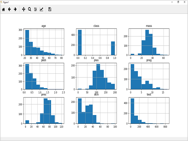
The above output shows that it created the histogram for each attribute in the dataset. From this, we can observe that perhaps age, pedi and test attribute may have exponential distribution while mass and plas have Gaussian distribution.
Density Plots
Another quick and easy technique for getting each attributes distribution is Density plots. It is also like histogram but having a smooth curve drawn through the top of each bin. We can call them as abstracted histograms.
Example
In the following example, Python script will generate Density Plots for the distribution of attributes of Pima Indian Diabetes dataset.
from matplotlib import pyplot
from pandas import read_csv
path = r"C:\pima-indians-diabetes.csv"
names = ['preg', 'plas', 'pres', 'skin', 'test', 'mass', 'pedi', 'age', 'class']
data = read_csv(path, names=names)
data.plot(kind='density', subplots=True, layout=(3,3), sharex=False)
pyplot.show()
Output
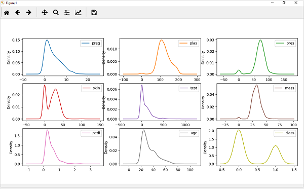
From the above output, the difference between Density plots and Histograms can be easily understood.
Box and Whisker Plots
Box and Whisker plots, also called boxplots in short, is another useful technique to review the distribution of each attributes distribution. The following are the characteristics of this technique −
It is univariate in nature and summarizes the distribution of each attribute.
It draws a line for the middle value i.e. for median.
It draws a box around the 25% and 75%.
It also draws whiskers which will give us an idea about the spread of the data.
The dots outside the whiskers signifies the outlier values. Outlier values would be 1.5 times greater than the size of the spread of the middle data.
Example
In the following example, Python script will generate Density Plots for the distribution of attributes of Pima Indian Diabetes dataset.
from matplotlib import pyplot
from pandas import read_csv
path = r"C:\pima-indians-diabetes.csv"
names = ['preg', 'plas', 'pres', 'skin', 'test', 'mass', 'pedi', 'age', 'class']
data = read_csv(path, names=names)
data.plot(kind='box', subplots=True, layout=(3,3), sharex=False,sharey=False)
pyplot.show()
Output
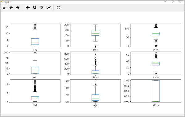
From the above plot of attributes distribution, it can be observed that age, test and skin appear skewed towards smaller values.
Multivariate Plots: Interaction Among Multiple Variables
Another type of visualization is multi-variable or multivariate visualization. With the help of multivariate visualization, we can understand interaction between multiple attributes of our dataset. The following are some techniques in Python to implement multivariate visualization −
Correlation Matrix Plot
Correlation is an indication about the changes between two variables. In our previous chapters, we have discussed Pearsons Correlation coefficients and the importance of Correlation too. We can plot correlation matrix to show which variable is having a high or low correlation in respect to another variable.
Example
In the following example, Python script will generate and plot correlation matrix for the Pima Indian Diabetes dataset. It can be generated with the help of corr() function on Pandas DataFrame and plotted with the help of pyplot.
from matplotlib import pyplot
from pandas import read_csv
import numpy
Path = r"C:\pima-indians-diabetes.csv"
names = ['preg', 'plas', 'pres', 'skin', 'test', 'mass', 'pedi', 'age', 'class']
data = read_csv(Path, names=names)
correlations = data.corr()
fig = pyplot.figure()
ax = fig.add_subplot(111)
cax = ax.matshow(correlations, vmin=-1, vmax=1)
fig.colorbar(cax)
ticks = numpy.arange(0,9,1)
ax.set_xticks(ticks)
ax.set_yticks(ticks)
ax.set_xticklabels(names)
ax.set_yticklabels(names)
pyplot.show()
Output
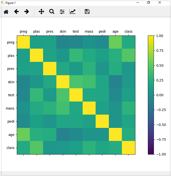
From the above output of correlation matrix, we can see that it is symmetrical i.e. the bottom left is same as the top right. It is also observed that each variable is positively correlated with each other.
Scatter Matrix Plot
Scatter plots shows how much one variable is affected by another or the relationship between them with the help of dots in two dimensions. Scatter plots are very much like line graphs in the concept that they use horizontal and vertical axes to plot data points.
Example
In the following example, Python script will generate and plot Scatter matrix for the Pima Indian Diabetes dataset. It can be generated with the help of scatter_matrix() function on Pandas DataFrame and plotted with the help of pyplot.
from matplotlib import pyplot
from pandas import read_csv
from pandas.tools.plotting import scatter_matrix
path = r"C:\pima-indians-diabetes.csv"
names = ['preg', 'plas', 'pres', 'skin', 'test', 'mass', 'pedi', 'age', 'class']
data = read_csv(path, names=names)
scatter_matrix(data)
pyplot.show()
Output

Machine Learning with Python - Preparing Data
Introduction
Machine Learning algorithms are completely dependent on data because it is the most crucial aspect that makes model training possible. On the other hand, if we wont be able to make sense out of that data, before feeding it to ML algorithms, a machine will be useless. In simple words, we always need to feed right data i.e. the data in correct scale, format and containing meaningful features, for the problem we want machine to solve.
This makes data preparation the most important step in ML process. Data preparation may be defined as the procedure that makes our dataset more appropriate for ML process.
Why Data Pre-processing?
After selecting the raw data for ML training, the most important task is data pre-processing. In broad sense, data preprocessing will convert the selected data into a form we can work with or can feed to ML algorithms. We always need to preprocess our data so that it can be as per the expectation of machine learning algorithm.
Data Pre-processing Techniques
We have the following data preprocessing techniques that can be applied on data set to produce data for ML algorithms −
Scaling
Most probably our dataset comprises of the attributes with varying scale, but we cannot provide such data to ML algorithm hence it requires rescaling. Data rescaling makes sure that attributes are at same scale. Generally, attributes are rescaled into the range of 0 and 1. ML algorithms like gradient descent and k-Nearest Neighbors requires scaled data. We can rescale the data with the help of MinMaxScaler class of scikit-learn Python library.
Example
In this example we will rescale the data of Pima Indians Diabetes dataset which we used earlier. First, the CSV data will be loaded (as done in the previous chapters) and then with the help of MinMaxScaler class, it will be rescaled in the range of 0 and 1.
The first few lines of the following script are same as we have written in previous chapters while loading CSV data.
from pandas import read_csv
from numpy import set_printoptions
from sklearn import preprocessing
path = r'C:\pima-indians-diabetes.csv'
names = ['preg', 'plas', 'pres', 'skin', 'test', 'mass', 'pedi', 'age', 'class']
dataframe = read_csv(path, names=names)
array = dataframe.values
Now, we can use MinMaxScaler class to rescale the data in the range of 0 and 1.
data_scaler = preprocessing.MinMaxScaler(feature_range=(0,1))
data_rescaled = data_scaler.fit_transform(array)
We can also summarize the data for output as per our choice. Here, we are setting the precision to 1 and showing the first 10 rows in the output.
set_printoptions(precision=1)
print ("\nScaled data:\n", data_rescaled[0:10])
Output
Scaled data:
[[0.4 0.7 0.6 0.4 0. 0.5 0.2 0.5 1. ]
[0.1 0.4 0.5 0.3 0. 0.4 0.1 0.2 0. ]
[0.5 0.9 0.5 0. 0. 0.3 0.3 0.2 1. ]
[0.1 0.4 0.5 0.2 0.1 0.4 0. 0. 0. ]
[0. 0.7 0.3 0.4 0.2 0.6 0.9 0.2 1. ]
[0.3 0.6 0.6 0. 0. 0.4 0.1 0.2 0. ]
[0.2 0.4 0.4 0.3 0.1 0.5 0.1 0.1 1. ]
[0.6 0.6 0. 0. 0. 0.5 0. 0.1 0. ]
[0.1 1. 0.6 0.5 0.6 0.5 0. 0.5 1. ]
[0.5 0.6 0.8 0. 0. 0. 0.1 0.6 1. ]]
From the above output, all the data got rescaled into the range of 0 and 1.
Normalization
Another useful data preprocessing technique is Normalization. This is used to rescale each row of data to have a length of 1. It is mainly useful in Sparse dataset where we have lots of zeros. We can rescale the data with the help of Normalizer class of scikit-learn Python library.
Types of Normalization
In machine learning, there are two types of normalization preprocessing techniques as follows −
L1 Normalization
It may be defined as the normalization technique that modifies the dataset values in a way that in each row the sum of the absolute values will always be up to 1. It is also called Least Absolute Deviations.
Example
In this example, we use L1 Normalize technique to normalize the data of Pima Indians Diabetes dataset which we used earlier. First, the CSV data will be loaded and then with the help of Normalizer class it will be normalized.
The first few lines of following script are same as we have written in previous chapters while loading CSV data.
from pandas import read_csv
from numpy import set_printoptions
from sklearn.preprocessing import Normalizer
path = r'C:\pima-indians-diabetes.csv'
names = ['preg', 'plas', 'pres', 'skin', 'test', 'mass', 'pedi', 'age', 'class']
dataframe = read_csv (path, names=names)
array = dataframe.values
Now, we can use Normalizer class with L1 to normalize the data.
Data_normalizer = Normalizer(norm='l1').fit(array)
Data_normalized = Data_normalizer.transform(array)
We can also summarize the data for output as per our choice. Here, we are setting the precision to 2 and showing the first 3 rows in the output.
set_printoptions(precision=2)
print ("\nNormalized data:\n", Data_normalized [0:3])
Output
Normalized data:
[[0.02 0.43 0.21 0.1 0. 0.1 0. 0.14 0. ]
[0. 0.36 0.28 0.12 0. 0.11 0. 0.13 0. ]
[0.03 0.59 0.21 0. 0. 0.07 0. 0.1 0. ]]
L2 Normalization
It may be defined as the normalization technique that modifies the dataset values in a way that in each row the sum of the squares will always be up to 1. It is also called least squares.
Example
In this example, we use L2 Normalization technique to normalize the data of Pima Indians Diabetes dataset which we used earlier. First, the CSV data will be loaded (as done in previous chapters) and then with the help of Normalizer class it will be normalized.
The first few lines of following script are same as we have written in previous chapters while loading CSV data.
from pandas import read_csv
from numpy import set_printoptions
from sklearn.preprocessing import Normalizer
path = r'C:\pima-indians-diabetes.csv'
names = ['preg', 'plas', 'pres', 'skin', 'test', 'mass', 'pedi', 'age', 'class']
dataframe = read_csv (path, names=names)
array = dataframe.values
Now, we can use Normalizer class with L1 to normalize the data.
Data_normalizer = Normalizer(norm='l2').fit(array)
Data_normalized = Data_normalizer.transform(array)
We can also summarize the data for output as per our choice. Here, we are setting the precision to 2 and showing the first 3 rows in the output.
set_printoptions(precision=2)
print ("\nNormalized data:\n", Data_normalized [0:3])
Output
Normalized data:
[[0.03 0.83 0.4 0.2 0. 0.19 0. 0.28 0.01]
[0.01 0.72 0.56 0.24 0. 0.22 0. 0.26 0. ]
[0.04 0.92 0.32 0. 0. 0.12 0. 0.16 0.01]]
Binarization
As the name suggests, this is the technique with the help of which we can make our data binary. We can use a binary threshold for making our data binary. The values above that threshold value will be converted to 1 and below that threshold will be converted to 0. For example, if we choose threshold value = 0.5, then the dataset value above it will become 1 and below this will become 0. That is why we can call it binarizing the data or thresholding the data. This technique is useful when we have probabilities in our dataset and want to convert them into crisp values.
We can binarize the data with the help of Binarizer class of scikit-learn Python library.
Example
In this example, we will rescale the data of Pima Indians Diabetes dataset which we used earlier. First, the CSV data will be loaded and then with the help of Binarizer class it will be converted into binary values i.e. 0 and 1 depending upon the threshold value. We are taking 0.5 as threshold value.
The first few lines of following script are same as we have written in previous chapters while loading CSV data.
from pandas import read_csv
from sklearn.preprocessing import Binarizer
path = r'C:\pima-indians-diabetes.csv'
names = ['preg', 'plas', 'pres', 'skin', 'test', 'mass', 'pedi', 'age', 'class']
dataframe = read_csv(path, names=names)
array = dataframe.values
Now, we can use Binarize class to convert the data into binary values.
binarizer = Binarizer(threshold=0.5).fit(array)
Data_binarized = binarizer.transform(array)
Here, we are showing the first 5 rows in the output.
print ("\nBinary data:\n", Data_binarized [0:5])
Output
Binary data:
[[1. 1. 1. 1. 0. 1. 1. 1. 1.]
[1. 1. 1. 1. 0. 1. 0. 1. 0.]
[1. 1. 1. 0. 0. 1. 1. 1. 1.]
[1. 1. 1. 1. 1. 1. 0. 1. 0.]
[0. 1. 1. 1. 1. 1. 1. 1. 1.]]
Standardization
Another useful data preprocessing technique which is basically used to transform the data attributes with a Gaussian distribution. It differs the mean and SD (Standard Deviation) to a standard Gaussian distribution with a mean of 0 and a SD of 1. This technique is useful in ML algorithms like linear regression, logistic regression that assumes a Gaussian distribution in input dataset and produce better results with rescaled data. We can standardize the data (mean = 0 and SD =1) with the help of StandardScaler class of scikit-learn Python library.
Example
In this example, we will rescale the data of Pima Indians Diabetes dataset which we used earlier. First, the CSV data will be loaded and then with the help of StandardScaler class it will be converted into Gaussian Distribution with mean = 0 and SD = 1.
The first few lines of following script are same as we have written in previous chapters while loading CSV data.
from sklearn.preprocessing import StandardScaler
from pandas import read_csv
from numpy import set_printoptions
path = r'C:\pima-indians-diabetes.csv'
names = ['preg', 'plas', 'pres', 'skin', 'test', 'mass', 'pedi', 'age', 'class']
dataframe = read_csv(path, names=names)
array = dataframe.values
Now, we can use StandardScaler class to rescale the data.
data_scaler = StandardScaler().fit(array)
data_rescaled = data_scaler.transform(array)
We can also summarize the data for output as per our choice. Here, we are setting the precision to 2 and showing the first 5 rows in the output.
set_printoptions(precision=2)
print ("\nRescaled data:\n", data_rescaled [0:5])
Output
Rescaled data:
[[ 0.64 0.85 0.15 0.91 -0.69 0.2 0.47 1.43 1.37]
[-0.84 -1.12 -0.16 0.53 -0.69 -0.68 -0.37 -0.19 -0.73]
[ 1.23 1.94 -0.26 -1.29 -0.69 -1.1 0.6 -0.11 1.37]
[-0.84 -1. -0.16 0.15 0.12 -0.49 -0.92 -1.04 -0.73]
[-1.14 0.5 -1.5 0.91 0.77 1.41 5.48 -0.02 1.37]]
Data Labeling
We discussed the importance of good fata for ML algorithms as well as some techniques to pre-process the data before sending it to ML algorithms. One more aspect in this regard is data labeling. It is also very important to send the data to ML algorithms having proper labeling. For example, in case of classification problems, lot of labels in the form of words, numbers etc. are there on the data.
What is Label Encoding?
Most of the sklearn functions expect that the data with number labels rather than word labels. Hence, we need to convert such labels into number labels. This process is called label encoding. We can perform label encoding of data with the help of LabelEncoder() function of scikit-learn Python library.
Example
In the following example, Python script will perform the label encoding.
First, import the required Python libraries as follows −
import numpy as np
from sklearn import preprocessing
Now, we need to provide the input labels as follows −
input_labels = ['red','black','red','green','black','yellow','white']
The next line of code will create the label encoder and train it.
encoder = preprocessing.LabelEncoder()
encoder.fit(input_labels)
The next lines of script will check the performance by encoding the random ordered list −
test_labels = ['green','red','black']
encoded_values = encoder.transform(test_labels)
print("\nLabels =", test_labels)
print("Encoded values =", list(encoded_values))
encoded_values = [3,0,4,1]
decoded_list = encoder.inverse_transform(encoded_values)
We can get the list of encoded values with the help of following python script −
print("\nEncoded values =", encoded_values)
print("\nDecoded labels =", list(decoded_list))
Output
Labels = ['green', 'red', 'black']
Encoded values = [1, 2, 0]
Encoded values = [3, 0, 4, 1]
Decoded labels = ['white', 'black', 'yellow', 'green']
ML with Python - Data Feature Selection
In the previous chapter, we have seen in detail how to preprocess and prepare data for machine learning. In this chapter, let us understand in detail data feature selection and various aspects involved in it.
Importance of Data Feature Selection
The performance of machine learning model is directly proportional to the data features used to train it. The performance of ML model will be affected negatively if the data features provided to it are irrelevant. On the other hand, use of relevant data features can increase the accuracy of your ML model especially linear and logistic regression.
Now the question arise that what is automatic feature selection? It may be defined as the process with the help of which we select those features in our data that are most relevant to the output or prediction variable in which we are interested. It is also called attribute selection.
The following are some of the benefits of automatic feature selection before modeling the data −
Performing feature selection before data modeling will reduce the overfitting.
Performing feature selection before data modeling will increases the accuracy of ML model.
Performing feature selection before data modeling will reduce the training time
Feature Selection Techniques
The followings are automatic feature selection techniques that we can use to model ML data in Python −
Univariate Selection
This feature selection technique is very useful in selecting those features, with the help of statistical testing, having strongest relationship with the prediction variables. We can implement univariate feature selection technique with the help of SelectKBest0class of scikit-learn Python library.
Example
In this example, we will use Pima Indians Diabetes dataset to select 4 of the attributes having best features with the help of chi-square statistical test.
from pandas import read_csv
from numpy import set_printoptions
from sklearn.feature_selection import SelectKBest
from sklearn.feature_selection import chi2
path = r'C:\pima-indians-diabetes.csv'
names = ['preg', 'plas', 'pres', 'skin', 'test', 'mass', 'pedi', 'age', 'class']
dataframe = read_csv(path, names=names)
array = dataframe.values
Next, we will separate array into input and output components −
X = array[:,0:8]
Y = array[:,8]
The following lines of code will select the best features from dataset −
test = SelectKBest(score_func=chi2, k=4)
fit = test.fit(X,Y)
We can also summarize the data for output as per our choice. Here, we are setting the precision to 2 and showing the 4 data attributes with best features along with best score of each attribute −
set_printoptions(precision=2)
print(fit.scores_)
featured_data = fit.transform(X)
print ("\nFeatured data:\n", featured_data[0:4])
Output
[ 111.52 1411.89 17.61 53.11 2175.57 127.67 5.39 181.3 ]
Featured data:
[[148. 0. 33.6 50. ]
[ 85. 0. 26.6 31. ]
[183. 0. 23.3 32. ]
[ 89. 94. 28.1 21. ]]
Recursive Feature Elimination
As the name suggests, RFE (Recursive feature elimination) feature selection technique removes the attributes recursively and builds the model with remaining attributes. We can implement RFE feature selection technique with the help of RFE class of scikit-learn Python library.
Example
In this example, we will use RFE with logistic regression algorithm to select the best 3 attributes having the best features from Pima Indians Diabetes dataset to.
from pandas import read_csv
from sklearn.feature_selection import RFE
from sklearn.linear_model import LogisticRegression
path = r'C:\pima-indians-diabetes.csv'
names = ['preg', 'plas', 'pres', 'skin', 'test', 'mass', 'pedi', 'age', 'class']
dataframe = read_csv(path, names=names)
array = dataframe.values
Next, we will separate the array into its input and output components −
X = array[:,0:8]
Y = array[:,8]
The following lines of code will select the best features from a dataset −
model = LogisticRegression()
rfe = RFE(model, 3)
fit = rfe.fit(X, Y)
print("Number of Features: %d")
print("Selected Features: %s")
print("Feature Ranking: %s")
Output
Number of Features: 3
Selected Features: [ True False False False False True True False]
Feature Ranking: [1 2 3 5 6 1 1 4]
We can see in above output, RFE choose preg, mass and pedi as the first 3 best features. They are marked as 1 in the output.
Principal Component Analysis (PCA)
PCA, generally called data reduction technique, is very useful feature selection technique as it uses linear algebra to transform the dataset into a compressed form. We can implement PCA feature selection technique with the help of PCA class of scikit-learn Python library. We can select number of principal components in the output.
Example
In this example, we will use PCA to select best 3 Principal components from Pima Indians Diabetes dataset.
from pandas import read_csv
from sklearn.decomposition import PCA
path = r'C:\pima-indians-diabetes.csv'
names = ['preg', 'plas', 'pres', 'skin', 'test', 'mass', 'pedi', 'age', 'class']
dataframe = read_csv(path, names=names)
array = dataframe.values
Next, we will separate array into input and output components −
X = array[:,0:8]
Y = array[:,8]
The following lines of code will extract features from dataset −
pca = PCA(n_components=3)
fit = pca.fit(X)
print("Explained Variance: %s") % fit.explained_variance_ratio_
print(fit.components_)
Output
Explained Variance: [ 0.88854663 0.06159078 0.02579012]
[[ -2.02176587e-03 9.78115765e-02 1.60930503e-02 6.07566861e-02
9.93110844e-01 1.40108085e-02 5.37167919e-04 -3.56474430e-03]
[ 2.26488861e-02 9.72210040e-01 1.41909330e-01 -5.78614699e-02
-9.46266913e-02 4.69729766e-02 8.16804621e-04 1.40168181e-01]
[ -2.24649003e-02 1.43428710e-01 -9.22467192e-01 -3.07013055e-01
2.09773019e-02 -1.32444542e-01 -6.39983017e-04 -1.25454310e-01]]
We can observe from the above output that 3 Principal Components bear little resemblance to the source data .
Feature Importance
As the name suggests, feature importance technique is used to choose the importance features. It basically uses a trained supervised classifier to select features. We can implement this feature selection technique with the help of ExtraTreeClassifier class of scikit-learn Python library.
Example
In this example, we will use ExtraTreeClassifier to select features from Pima Indians Diabetes dataset.
from pandas import read_csv
from sklearn.ensemble import ExtraTreesClassifier
path = r'C:\Desktop\pima-indians-diabetes.csv'
names = ['preg', 'plas', 'pres', 'skin', 'test', 'mass', 'pedi', 'age', 'class']
dataframe = read_csv(data, names=names)
array = dataframe.values
Next, we will separate array into input and output components −
X = array[:,0:8]
Y = array[:,8]
The following lines of code will extract features from dataset −
model = ExtraTreesClassifier()
model.fit(X, Y)
print(model.feature_importances_)
Output
[ 0.11070069 0.2213717 0.08824115 0.08068703 0.07281761 0.14548537 0.12654214 0.15415431]
From the output, we can observe that there are scores for each attribute. The higher the score, higher is the importance of that attribute.
Classification - Introduction
Introduction to Classification
Classification may be defined as the process of predicting class or category from observed values or given data points. The categorized output can have the form such as Black or White or spam or no spam.
Mathematically, classification is the task of approximating a mapping function (f) from input variables (X) to output variables (Y). It is basically belongs to the supervised machine learning in which targets are also provided along with the input data set.
An example of classification problem can be the spam detection in emails. There can be only two categories of output, spam and no spam; hence this is a binary type classification.
To implement this classification, we first need to train the classifier. For this example, spam and no spam emails would be used as the training data. After successfully train the classifier, it can be used to detect an unknown email.
Types of Learners in Classification
We have two types of learners in respective to classification problems −
Lazy Learners
As the name suggests, such kind of learners waits for the testing data to be appeared after storing the training data. Classification is done only after getting the testing data. They spend less time on training but more time on predicting. Examples of lazy learners are K-nearest neighbor and case-based reasoning.
Eager Learners
As opposite to lazy learners, eager learners construct classification model without waiting for the testing data to be appeared after storing the training data. They spend more time on training but less time on predicting. Examples of eager learners are Decision Trees, Nave Bayes and Artificial Neural Networks (ANN).
Building a Classifier in Python
Scikit-learn, a Python library for machine learning can be used to build a classifier in Python. The steps for building a classifier in Python are as follows −
Step1: Importing necessary python package
For building a classifier using scikit-learn, we need to import it. We can import it by using following script −
import sklearn
Step2: Importing dataset
After importing necessary package, we need a dataset to build classification prediction model. We can import it from sklearn dataset or can use other one as per our requirement. We are going to use sklearns Breast Cancer Wisconsin Diagnostic Database. We can import it with the help of following script −
from sklearn.datasets import load_breast_cancer
The following script will load the dataset;
data = load_breast_cancer()
We also need to organize the data and it can be done with the help of following scripts −
label_names = data['target_names']
   labels = data['target']
   feature_names = data['feature_names']
   features = data['data']
The following command will print the name of the labels, malignant and benign in case of our database.
print(label_names)
The output of the above command is the names of the labels −
['malignant' 'benign']
These labels are mapped to binary values 0 and 1. Malignant cancer is represented by 0 and Benign cancer is represented by 1.
The feature names and feature values of these labels can be seen with the help of following commands −
print(feature_names[0])
The output of the above command is the names of the features for label 0 i.e. Malignant cancer −
mean radius
Similarly, names of the features for label can be produced as follows −
print(feature_names[1])
The output of the above command is the names of the features for label 1 i.e. Benign cancer −
mean texture
We can print the features for these labels with the help of following command −
print(features[0])
This will give the following output −
[1.799e+01 1.038e+01 1.228e+02 1.001e+03 1.184e-01 2.776e-01 3.001e-01
1.471e-01 2.419e-01 7.871e-02 1.095e+00 9.053e-01 8.589e+00 1.534e+02
6.399e-03 4.904e-02 5.373e-02 1.587e-02 3.003e-02 6.193e-03 2.538e+01
1.733e+01 1.846e+02 2.019e+03 1.622e-01 6.656e-01 7.119e-01 2.654e-01
4.601e-01 1.189e-01]
We can print the features for these labels with the help of following command −
print(features[1])
This will give the following output −
[2.057e+01 1.777e+01 1.329e+02 1.326e+03 8.474e-02 7.864e-02 8.690e-02
7.017e-02 1.812e-01 5.667e-02 5.435e-01 7.339e-01 3.398e+00 7.408e+01
5.225e-03 1.308e-02 1.860e-02 1.340e-02 1.389e-02 3.532e-03 2.499e+01
2.341e+01 1.588e+02 1.956e+03 1.238e-01 1.866e-01 2.416e-01 1.860e-01
2.750e-01 8.902e-02]
Step3: Organizing data into training & testing sets
As we need to test our model on unseen data, we will divide our dataset into two parts: a training set and a test set. We can use train_test_split() function of sklearn python package to split the data into sets. The following command will import the function −
from sklearn.model_selection import train_test_split
Now, next command will split the data into training & testing data. In this example, we are using taking 40 percent of the data for testing purpose and 60 percent of the data for training purpose −
train, test, train_labels, test_labels = train_test_split(features,labels,test_size = 0.40, random_state = 42)
Step4 - Model evaluation
After dividing the data into training and testing we need to build the model. We will be using Nave Bayes algorithm for this purpose. The following commands will import the GaussianNB module −
from sklearn.naive_bayes import GaussianNB
Now, initialize the model as follows −
gnb = GaussianNB()
Next, with the help of following command we can train the model −
model = gnb.fit(train, train_labels)
Now, for evaluation purpose we need to make predictions. It can be done by using predict() function as follows −
preds = gnb.predict(test)
print(preds)
This will give the following output −
[1 0 0 1 1 0 0 0 1 1 1 0 1 0 1 0 1 1 1 0 1 1 0 1 1 1 1 1 1 0 1 1 1 1 1 1 0
1 0 1 1 0 1 1 1 1 1 1 1 1 0 0 1 1 1 1 1 0 0 1 1 0 0 1 1 1 0 0 1 1 0 0 1 0
1 1 1 1 1 1 0 1 1 0 0 0 0 0 1 1 1 1 1 1 1 1 0 0 1 0 0 1 0 0 1 1 1 0 1 1 0
1 1 0 0 0 1 1 1 0 0 1 1 0 1 0 0 1 1 0 0 0 1 1 1 0 1 1 0 0 1 0 1 1 0 1 0 0
1 1 1 1 1 1 1 0 0 1 1 1 1 1 1 1 1 1 1 1 1 0 1 1 1 0 1 1 0 1 1 1 1 1 1 0 0
0 1 1 0 1 0 1 1 1 1 0 1 1 0 1 1 1 0 1 0 0 1 1 1 1 1 1 1 1 0 1 1 1 1 1 0 1
0 0 1 1 0 1]
The above series of 0s and 1s in output are the predicted values for the Malignant and Benign tumor classes.
Step5- Finding accuracy
We can find the accuracy of the model build in previous step by comparing the two arrays namely test_labels and preds. We will be using the accuracy_score() function to determine the accuracy.
from sklearn.metrics import accuracy_score
   print(accuracy_score(test_labels,preds))
   0.951754385965
The above output shows that NaveBayes classifier is 95.17% accurate .
Classification Evaluation Metrics
The job is not done even if you have finished implementation of your Machine Learning application or model. We must have to find out how effective our model is? There can be different evaluation metrics, but we must choose it carefully because the choice of metrics influences how the performance of a machine learning algorithm is measured and compared.
The following are some of the important classification evaluation metrics among which you can choose based upon your dataset and kind of problem −
Confusion Matrix
It is the easiest way to measure the performance of a classification problem where the output can be of two or more type of classes. A confusion matrix is nothing but a table with two dimensions viz. Actual and Predicted and furthermore, both the dimensions have True Positives (TP), True Negatives (TN), False Positives (FP), False Negatives (FN) as shown below −
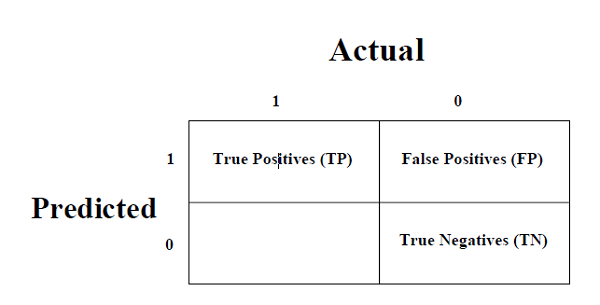
True Positives (TP) − It is the case when both actual class & predicted class of data point is 1.
True Negatives (TN) − It is the case when both actual class & predicted class of data point is 0.
False Positives (FP) − It is the case when actual class of data point is 0 & predicted class of data point is 1.
False Negatives (FN) − It is the case when actual class of data point is 1 & predicted class of data point is 0.
We can find the confusion matrix with the help of confusion_matrix() function of sklearn. With the help of the following script, we can find the confusion matrix of above built binary classifier −
from sklearn.metrics import confusion_matrix
Output
[[ 73 7]
[ 4 144]]
Accuracy
It may be defined as the number of correct predictions made by our ML model. We can easily calculate it by confusion matrix with the help of following formula −
$$=\frac{+}{+++}$$For above built binary classifier, TP + TN = 73+144 = 217 and TP+FP+FN+TN = 73+7+4+144=228.
Hence, Accuracy = 217/228 = 0.951754385965 which is same as we have calculated after creating our binary classifier.
Precision
Precision, used in document retrievals, may be defined as the number of correct documents returned by our ML model. We can easily calculate it by confusion matrix with the help of following formula −
$$=\frac{}{+FP}$$For the above built binary classifier, TP = 73 and TP+FP = 73+7 = 80.
Hence, Precision = 73/80 = 0.915
Recall or Sensitivity
Recall may be defined as the number of positives returned by our ML model. We can easily calculate it by confusion matrix with the help of following formula −
$$=\frac{}{+FN}$$For above built binary classifier, TP = 73 and TP+FN = 73+4 = 77.
Hence, Precision = 73/77 = 0.94805
Specificity
Specificity, in contrast to recall, may be defined as the number of negatives returned by our ML model. We can easily calculate it by confusion matrix with the help of following formula −
$$=\frac{N}{N+FP}$$For the above built binary classifier, TN = 144 and TN+FP = 144+7 = 151.
Hence, Precision = 144/151 = 0.95364
Various ML Classification Algorithms
The followings are some important ML classification algorithms −
Logistic Regression
Support Vector Machine (SVM)
Decision Tree
Nave Bayes
Random Forest
We will be discussing all these classification algorithms in detail in further chapters.
Applications
Some of the most important applications of classification algorithms are as follows −
Speech Recognition
Handwriting Recognition
Biometric Identification
Document Classification
Classification Algorithms - Logistic Regression
Introduction to Logistic Regression
Logistic regression is a supervised learning classification algorithm used to predict the probability of a target variable. The nature of target or dependent variable is dichotomous, which means there would be only two possible classes.
In simple words, the dependent variable is binary in nature having data coded as either 1 (stands for success/yes) or 0 (stands for failure/no).
Mathematically, a logistic regression model predicts P(Y=1) as a function of X. It is one of the simplest ML algorithms that can be used for various classification problems such as spam detection, Diabetes prediction, cancer detection etc.
Types of Logistic Regression
Generally, logistic regression means binary logistic regression having binary target variables, but there can be two more categories of target variables that can be predicted by it. Based on those number of categories, Logistic regression can be divided into following types −
Binary or Binomial
In such a kind of classification, a dependent variable will have only two possible types either 1 and 0. For example, these variables may represent success or failure, yes or no, win or loss etc.
Multinomial
In such a kind of classification, dependent variable can have 3 or more possible unordered types or the types having no quantitative significance. For example, these variables may represent Type A or Type B or Type C.
Ordinal
In such a kind of classification, dependent variable can have 3 or more possible ordered types or the types having a quantitative significance. For example, these variables may represent poor or good, very good, Excellent and each category can have the scores like 0,1,2,3.
Logistic Regression Assumptions
Before diving into the implementation of logistic regression, we must be aware of the following assumptions about the same −
In case of binary logistic regression, the target variables must be binary always and the desired outcome is represented by the factor level 1.
There should not be any multi-collinearity in the model, which means the independent variables must be independent of each other .
We must include meaningful variables in our model.
We should choose a large sample size for logistic regression.
Binary Logistic Regression model
The simplest form of logistic regression is binary or binomial logistic regression in which the target or dependent variable can have only 2 possible types either 1 or 0. It allows us to model a relationship between multiple predictor variables and a binary/binomial target variable. In case of logistic regression, the linear function is basically used as an input to another function such as in the following relation −
$h_{\theta}{(x)}=g(\theta^{T}x) 0h_{\theta}1$Here, is the logistic or sigmoid function which can be given as follows −
$g(z)= \frac{1}{1+e^{-z}} =\theta ^{T}$To sigmoid curve can be represented with the help of following graph. We can see the values of y-axis lie between 0 and 1 and crosses the axis at 0.5.
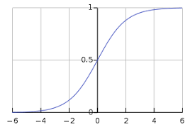
The classes can be divided into positive or negative. The output comes under the probability of positive class if it lies between 0 and 1. For our implementation, we are interpreting the output of hypothesis function as positive if it is 0.5, otherwise negative.
We also need to define a loss function to measure how well the algorithm performs using the weights on functions, represented by theta as follows −
=()
$J(\theta) = \frac{1}{m}.(-y^{T}log(h) - (1 -y)^Tlog(1-h))$Now, after defining the loss function our prime goal is to minimize the loss function. It can be done with the help of fitting the weights which means by increasing or decreasing the weights. With the help of derivatives of the loss function w.r.t each weight, we would be able to know what parameters should have high weight and what should have smaller weight.
The following gradient descent equation tells us how loss would change if we modified the parameters −
$\frac{()}{\theta_{j}}=\frac{1}{m}X^{T}(())$Implementation in Python
Now we will implement the above concept of binomial logistic regression in Python. For this purpose, we are using a multivariate flower dataset named iris which have 3 classes of 50 instances each, but we will be using the first two feature columns. Every class represents a type of iris flower.
First, we need to import the necessary libraries as follows −
import numpy as np
import matplotlib.pyplot as plt
import seaborn as sns
from sklearn import datasets
Next, load the iris dataset as follows −
iris = datasets.load_iris()
X = iris.data[:, :2]
y = (iris.target != 0) * 1
We can plot our training data s follows −
plt.figure(figsize=(6, 6))
plt.scatter(X[y == 0][:, 0], X[y == 0][:, 1], color='g', label='0')
plt.scatter(X[y == 1][:, 0], X[y == 1][:, 1], color='y', label='1')
plt.legend();
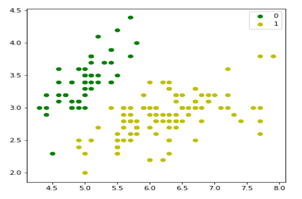
Next, we will define sigmoid function, loss function and gradient descend as follows −
class LogisticRegression:
   def __init__(self, lr=0.01, num_iter=100000, fit_intercept=True, verbose=False):
      self.lr = lr
      self.num_iter = num_iter
      self.fit_intercept = fit_intercept
      self.verbose = verbose
   def __add_intercept(self, X):
      intercept = np.ones((X.shape[0], 1))
      return np.concatenate((intercept, X), axis=1)
   def __sigmoid(self, z):
      return 1 / (1 + np.exp(-z))
   def __loss(self, h, y):
      return (-y * np.log(h) - (1 - y) * np.log(1 - h)).mean()
   def fit(self, X, y):
      if self.fit_intercept:
         X = self.__add_intercept(X)
Now, initialize the weights as follows −
self.theta = np.zeros(X.shape[1])
   for i in range(self.num_iter):
      z = np.dot(X, self.theta)
      h = self.__sigmoid(z)
      gradient = np.dot(X.T, (h - y)) / y.size
      self.theta -= self.lr * gradient
      z = np.dot(X, self.theta)
      h = self.__sigmoid(z)
      loss = self.__loss(h, y)
      if(self.verbose ==True and i % 10000 == 0):
         print(f'loss: {loss} \t')
With the help of the following script, we can predict the output probabilities −
def predict_prob(self, X):
   if self.fit_intercept:
      X = self.__add_intercept(X)
   return self.__sigmoid(np.dot(X, self.theta))
def predict(self, X):
   return self.predict_prob(X).round()
Next, we can evaluate the model and plot it as follows −
model = LogisticRegression(lr=0.1, num_iter=300000)
preds = model.predict(X)
(preds == y).mean()

plt.figure(figsize=(10, 6))
plt.scatter(X[y == 0][:, 0], X[y == 0][:, 1], color='g', label='0')
plt.scatter(X[y == 1][:, 0], X[y == 1][:, 1], color='y', label='1')
plt.legend()
x1_min, x1_max = X[:,0].min(), X[:,0].max(),
x2_min, x2_max = X[:,1].min(), X[:,1].max(),
xx1, xx2 = np.meshgrid(np.linspace(x1_min, x1_max), np.linspace(x2_min, x2_max))
grid = np.c_[xx1.ravel(), xx2.ravel()]
probs = model.predict_prob(grid).reshape(xx1.shape)
plt.contour(xx1, xx2, probs, [0.5], linewidths=1, colors='red');
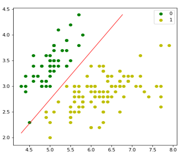
Multinomial Logistic Regression Model
Another useful form of logistic regression is multinomial logistic regression in which the target or dependent variable can have 3 or more possible unordered types i.e. the types having no quantitative significance.
Implementation in Python
Now we will implement the above concept of multinomial logistic regression in Python. For this purpose, we are using a dataset from sklearn named digit.
First, we need to import the necessary libraries as follows −
Import sklearn
from sklearn import datasets
from sklearn import linear_model
from sklearn import metrics
from sklearn.model_selection import train_test_split
Next, we need to load digit dataset −
digits = datasets.load_digits()
Now, define the feature matrix(X) and response vector(y)as follows −
X = digits.data
y = digits.target
With the help of next line of code, we can split X and y into training and testing sets −
X_train, X_test, y_train, y_test = train_test_split(X, y, test_size=0.4, random_state=1)
Now create an object of logistic regression as follows −
digreg = linear_model.LogisticRegression()
Now, we need to train the model by using the training sets as follows −
digreg.fit(X_train, y_train)
Next, make the predictions on testing set as follows −
y_pred = digreg.predict(X_test)
Next print the accuracy of the model as follows −
print("Accuracy of Logistic Regression model is:",
metrics.accuracy_score(y_test, y_pred)*100)
Output
Accuracy of Logistic Regression model is: 95.6884561891516
From the above output we can see the accuracy of our model is around 96 percent.
Support Vector Machine (SVM)
Introduction to SVM
Support vector machines (SVMs) are powerful yet flexible supervised machine learning algorithms which are used both for classification and regression. But generally, they are used in classification problems. In 1960s, SVMs were first introduced but later they got refined in 1990. SVMs have their unique way of implementation as compared to other machine learning algorithms. Lately, they are extremely popular because of their ability to handle multiple continuous and categorical variables.
Working of SVM
An SVM model is basically a representation of different classes in a hyperplane in multidimensional space. The hyperplane will be generated in an iterative manner by SVM so that the error can be minimized. The goal of SVM is to divide the datasets into classes to find a maximum marginal hyperplane (MMH).
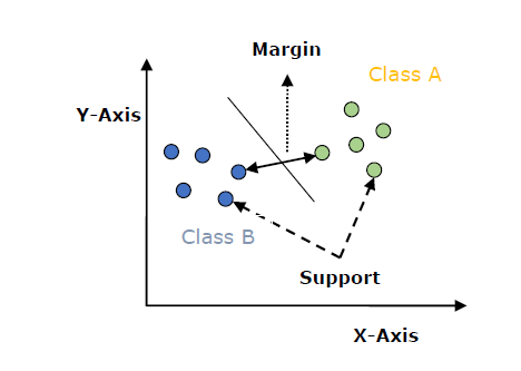
The followings are important concepts in SVM −
Support Vectors − Datapoints that are closest to the hyperplane is called support vectors. Separating line will be defined with the help of these data points.
Hyperplane − As we can see in the above diagram, it is a decision plane or space which is divided between a set of objects having different classes.
Margin − It may be defined as the gap between two lines on the closet data points of different classes. It can be calculated as the perpendicular distance from the line to the support vectors. Large margin is considered as a good margin and small margin is considered as a bad margin.
The main goal of SVM is to divide the datasets into classes to find a maximum marginal hyperplane (MMH) and it can be done in the following two steps −
First, SVM will generate hyperplanes iteratively that segregates the classes in best way.
Then, it will choose the hyperplane that separates the classes correctly.
Implementing SVM in Python
For implementing SVM in Python we will start with the standard libraries import as follows −
import numpy as np
import matplotlib.pyplot as plt
from scipy import stats
import seaborn as sns; sns.set()
Next, we are creating a sample dataset, having linearly separable data, from sklearn.dataset.sample_generator for classification using SVM −
from sklearn.datasets.samples_generator import make_blobs
X, y = make_blobs(n_samples=100, centers=2,
      random_state=0, cluster_std=0.50)
plt.scatter(X[:, 0], X[:, 1], c=y, s=50, cmap='summer');
The following would be the output after generating sample dataset having 100 samples and 2 clusters −
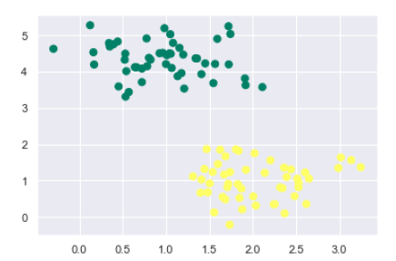
We know that SVM supports discriminative classification. it divides the classes from each other by simply finding a line in case of two dimensions or manifold in case of multiple dimensions. It is implemented on the above dataset as follows −
xfit = np.linspace(-1, 3.5)
plt.scatter(X[:, 0], X[:, 1], c=y, s=50, cmap='summer')
plt.plot([0.6], [2.1], 'x', color='black', markeredgewidth=4, markersize=12)
for m, b in [(1, 0.65), (0.5, 1.6), (-0.2, 2.9)]:
   plt.plot(xfit, m * xfit + b, '-k')
plt.xlim(-1, 3.5);
The output is as follows −
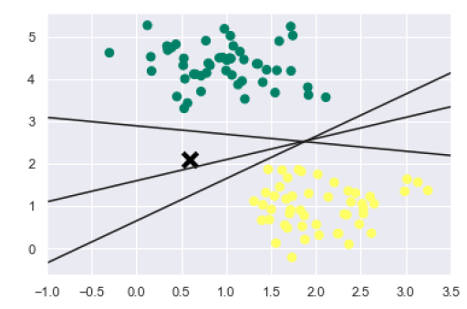
We can see from the above output that there are three different separators that perfectly discriminate the above samples.
As discussed, the main goal of SVM is to divide the datasets into classes to find a maximum marginal hyperplane (MMH) hence rather than drawing a zero line between classes we can draw around each line a margin of some width up to the nearest point. It can be done as follows −
xfit = np.linspace(-1, 3.5)
plt.scatter(X[:, 0], X[:, 1], c=y, s=50, cmap='summer')
   for m, b, d in [(1, 0.65, 0.33), (0.5, 1.6, 0.55), (-0.2, 2.9, 0.2)]:
   yfit = m * xfit + b
   plt.plot(xfit, yfit, '-k')
   plt.fill_between(xfit, yfit - d, yfit + d, edgecolor='none',
         color='#AAAAAA', alpha=0.4)
plt.xlim(-1, 3.5);
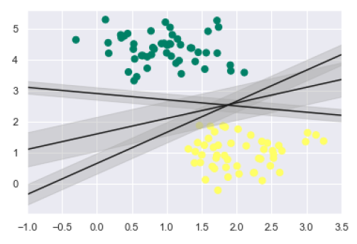
From the above image in output, we can easily observe the margins within the discriminative classifiers. SVM will choose the line that maximizes the margin.
Next, we will use Scikit-Learns support vector classifier to train an SVM model on this data. Here, we are using linear kernel to fit SVM as follows −
from sklearn.svm import SVC # "Support vector classifier"
model = SVC(kernel='linear', C=1E10)
model.fit(X, y)
The output is as follows −
SVC(C=10000000000.0, cache_size=200, class_weight=None, coef0=0.0,
decision_function_shape='ovr', degree=3, gamma='auto_deprecated',
kernel='linear', max_iter=-1, probability=False, random_state=None,
shrinking=True, tol=0.001, verbose=False)
Now, for a better understanding, the following will plot the decision functions for 2D SVC −
def decision_function(model, ax=None, plot_support=True):
   if ax is None:
      ax = plt.gca()
   xlim = ax.get_xlim()
   ylim = ax.get_ylim()
For evaluating model, we need to create grid as follows −
x = np.linspace(xlim[0], xlim[1], 30)
y = np.linspace(ylim[0], ylim[1], 30)
Y, X = np.meshgrid(y, x)
xy = np.vstack([X.ravel(), Y.ravel()]).T
P = model.decision_function(xy).reshape(X.shape)
Next, we need to plot decision boundaries and margins as follows −
ax.contour(X, Y, P, colors='k',
   levels=[-1, 0, 1], alpha=0.5,
   linestyles=['--', '-', '--'])
Now, similarly plot the support vectors as follows −
if plot_support:
   ax.scatter(model.support_vectors_[:, 0],
      model.support_vectors_[:, 1],
      s=300, linewidth=1, facecolors='none');
ax.set_xlim(xlim)
ax.set_ylim(ylim)
Now, use this function to fit our models as follows −
plt.scatter(X[:, 0], X[:, 1], c=y, s=50, cmap='summer')
decision_function(model);
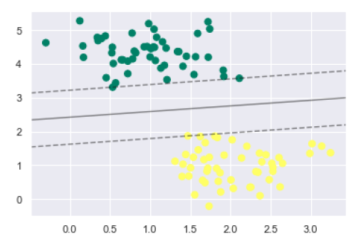
We can observe from the above output that an SVM classifier fit to the data with margins i.e. dashed lines and support vectors, the pivotal elements of this fit, touching the dashed line. These support vector points are stored in the support_vectors_ attribute of the classifier as follows −
model.support_vectors_
The output is as follows −
array([[0.5323772 , 3.31338909],
   [2.11114739, 3.57660449],
   [1.46870582, 1.86947425]])
SVM Kernels
In practice, SVM algorithm is implemented with kernel that transforms an input data space into the required form. SVM uses a technique called the kernel trick in which kernel takes a low dimensional input space and transforms it into a higher dimensional space. In simple words, kernel converts non-separable problems into separable problems by adding more dimensions to it. It makes SVM more powerful, flexible and accurate. The following are some of the types of kernels used by SVM −
Linear Kernel
It can be used as a dot product between any two observations. The formula of linear kernel is as below −
k(x,xi) = sum(x*xi)
From the above formula, we can see that the product between two vectors say & is the sum of the multiplication of each pair of input values.
Polynomial Kernel
It is more generalized form of linear kernel and distinguish curved or nonlinear input space. Following is the formula for polynomial kernel −
K(x, xi) = 1 + sum(x * xi)^d
Here d is the degree of polynomial, which we need to specify manually in the learning algorithm.
Radial Basis Function (RBF) Kernel
RBF kernel, mostly used in SVM classification, maps input space in indefinite dimensional space. Following formula explains it mathematically −
K(x,xi) = exp(-gamma * sum((x xi^2))
Here, gamma ranges from 0 to 1. We need to manually specify it in the learning algorithm. A good default value of gamma is 0.1.
As we implemented SVM for linearly separable data, we can implement it in Python for the data that is not linearly separable. It can be done by using kernels.
Example
The following is an example for creating an SVM classifier by using kernels. We will be using iris dataset from scikit-learn −
We will start by importing following packages −
import pandas as pd
import numpy as np
from sklearn import svm, datasets
import matplotlib.pyplot as plt
Now, we need to load the input data −
iris = datasets.load_iris()
From this dataset, we are taking first two features as follows −
X = iris.data[:, :2]
y = iris.target
Next, we will plot the SVM boundaries with original data as follows −
x_min, x_max = X[:, 0].min() - 1, X[:, 0].max() + 1
y_min, y_max = X[:, 1].min() - 1, X[:, 1].max() + 1
h = (x_max / x_min)/100
xx, yy = np.meshgrid(np.arange(x_min, x_max, h),
   np.arange(y_min, y_max, h))
X_plot = np.c_[xx.ravel(), yy.ravel()]
Now, we need to provide the value of regularization parameter as follows −
C = 1.0
Next, SVM classifier object can be created as follows −
Svc_classifier = svm.SVC(kernel='linear', C=C).fit(X, y)
Z = svc_classifier.predict(X_plot)
Z = Z.reshape(xx.shape)
plt.figure(figsize=(15, 5))
plt.subplot(121)
plt.contourf(xx, yy, Z, cmap=plt.cm.tab10, alpha=0.3)
plt.scatter(X[:, 0], X[:, 1], c=y, cmap=plt.cm.Set1)
plt.xlabel('Sepal length')
plt.ylabel('Sepal width')
plt.xlim(xx.min(), xx.max())
plt.title('Support Vector Classifier with linear kernel')
Output
Text(0.5, 1.0, 'Support Vector Classifier with linear kernel')
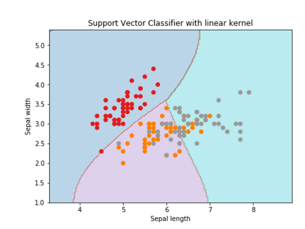
For creating SVM classifier with rbf kernel, we can change the kernel to rbf as follows −
Svc_classifier = svm.SVC(kernel='rbf', gamma =auto,C=C).fit(X, y)
Z = svc_classifier.predict(X_plot)
Z = Z.reshape(xx.shape)
plt.figure(figsize=(15, 5))
plt.subplot(121)
plt.contourf(xx, yy, Z, cmap=plt.cm.tab10, alpha=0.3)
plt.scatter(X[:, 0], X[:, 1], c=y, cmap=plt.cm.Set1)
plt.xlabel('Sepal length')
plt.ylabel('Sepal width')
plt.xlim(xx.min(), xx.max())
plt.title('Support Vector Classifier with rbf kernel')
Output
Text(0.5, 1.0, 'Support Vector Classifier with rbf kernel')
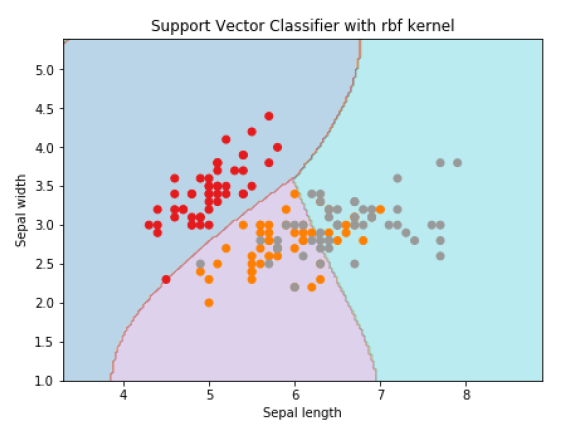
We put the value of gamma to auto but you can provide its value between 0 to 1 also.
Pros and Cons of SVM Classifiers
Pros of SVM classifiers
SVM classifiers offers great accuracy and work well with high dimensional space. SVM classifiers basically use a subset of training points hence in result uses very less memory.
Cons of SVM classifiers
They have high training time hence in practice not suitable for large datasets. Another disadvantage is that SVM classifiers do not work well with overlapping classes.
Classification Algorithms - Decision Tree
Introduction to Decision Tree
In general, Decision tree analysis is a predictive modelling tool that can be applied across many areas. Decision trees can be constructed by an algorithmic approach that can split the dataset in different ways based on different conditions. Decisions tress are the most powerful algorithms that falls under the category of supervised algorithms.
They can be used for both classification and regression tasks. The two main entities of a tree are decision nodes, where the data is split and leaves, where we got outcome. The example of a binary tree for predicting whether a person is fit or unfit providing various information like age, eating habits and exercise habits, is given below −
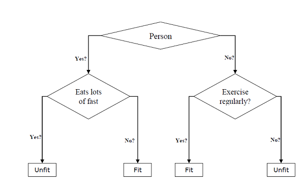
In the above decision tree, the question are decision nodes and final outcomes are leaves. We have the following two types of decision trees −
Classification decision trees − In this kind of decision trees, the decision variable is categorical. The above decision tree is an example of classification decision tree.
Regression decision trees − In this kind of decision trees, the decision variable is continuous.
Implementing Decision Tree Algorithm
Gini Index
It is the name of the cost function that is used to evaluate the binary splits in the dataset and works with the categorial target variable Success or Failure.
Higher the value of Gini index, higher the homogeneity. A perfect Gini index value is 0 and worst is 0.5 (for 2 class problem). Gini index for a split can be calculated with the help of following steps −
First, calculate Gini index for sub-nodes by using the formula p^2+q^2 , which is the sum of the square of probability for success and failure.
Next, calculate Gini index for split using weighted Gini score of each node of that split.
Classification and Regression Tree (CART) algorithm uses Gini method to generate binary splits.
Split Creation
A split is basically including an attribute in the dataset and a value. We can create a split in dataset with the help of following three parts −
Part1 − Calculating Gini Score: We have just discussed this part in the previous section.
Part2 − Splitting a dataset: It may be defined as separating a dataset into two lists of rows having index of an attribute and a split value of that attribute. After getting the two groups - right and left, from the dataset, we can calculate the value of split by using Gini score calculated in first part. Split value will decide in which group the attribute will reside.
Part3 − Evaluating all splits: Next part after finding Gini score and splitting dataset is the evaluation of all splits. For this purpose, first, we must check every value associated with each attribute as a candidate split. Then we need to find the best possible split by evaluating the cost of the split. The best split will be used as a node in the decision tree.
Building a Tree
As we know that a tree has root node and terminal nodes. After creating the root node, we can build the tree by following two parts −
Part1: Terminal node creation
While creating terminal nodes of decision tree, one important point is to decide when to stop growing tree or creating further terminal nodes. It can be done by using two criteria namely maximum tree depth and minimum node records as follows −
Maximum Tree Depth − As name suggests, this is the maximum number of the nodes in a tree after root node. We must stop adding terminal nodes once a tree reached at maximum depth i.e. once a tree got maximum number of terminal nodes.
Minimum Node Records − It may be defined as the minimum number of training patterns that a given node is responsible for. We must stop adding terminal nodes once tree reached at these minimum node records or below this minimum.
Terminal node is used to make a final prediction.
Part2: Recursive Splitting
As we understood about when to create terminal nodes, now we can start building our tree. Recursive splitting is a method to build the tree. In this method, once a node is created, we can create the child nodes (nodes added to an existing node) recursively on each group of data, generated by splitting the dataset, by calling the same function again and again.
Prediction
After building a decision tree, we need to make a prediction about it. Basically, prediction involves navigating the decision tree with the specifically provided row of data.
We can make a prediction with the help of recursive function, as did above. The same prediction routine is called again with the left or the child right nodes.
Assumptions
The following are some of the assumptions we make while creating decision tree −
While preparing decision trees, the training set is as root node.
Decision tree classifier prefers the features values to be categorical. In case if you want to use continuous values then they must be done discretized prior to model building.
Based on the attributes values, the records are recursively distributed.
Statistical approach will be used to place attributes at any node position i.e.as root node or internal node.
Implementation in Python
Example
In the following example, we are going to implement Decision Tree classifier on Pima Indian Diabetes −
First, start with importing necessary python packages −
import pandas as pd
from sklearn.tree import DecisionTreeClassifier
from sklearn.model_selection import train_test_split
Next, download the iris dataset from its weblink as follows −
col_names = ['pregnant', 'glucose', 'bp', 'skin', 'insulin', 'bmi', 'pedigree', 'age', 'label']
pima = pd.read_csv(r"C:\pima-indians-diabetes.csv", header=None, names=col_names)
pima.head()
      pregnant    glucose  bp    skin  insulin  bmi   pedigree    age   label
0       6         148      72    35     0       33.6    0.627     50      1
1       1         85       66    29     0       26.6    0.351     31      0
2       8         183      64     0     0       23.3    0.672     32      1
3       1         89       66    23     94      28.1    0.167     21      0
4       0         137      40    35     168     43.1    2.288     33      1
Now, split the dataset into features and target variable as follows −
feature_cols = ['pregnant', 'insulin', 'bmi', 'age','glucose','bp','pedigree']
X = pima[feature_cols] # Features
y = pima.label # Target variable
Next, we will divide the data into train and test split. The following code will split the dataset into 70% training data and 30% of testing data −
X_train, X_test, y_train, y_test = train_test_split(X, y, test_size=0.3, random_state=1)
Next, train the model with the help of DecisionTreeClassifier class of sklearn as follows −
clf = DecisionTreeClassifier()
clf = clf.fit(X_train,y_train)
At last we need to make prediction. It can be done with the help of following script −
y_pred = clf.predict(X_test)
Next, we can get the accuracy score, confusion matrix and classification report as follows −
from sklearn.metrics import classification_report, confusion_matrix, accuracy_score
result = confusion_matrix(y_test, y_pred)
print("Confusion Matrix:")
print(result)
result1 = classification_report(y_test, y_pred)
print("Classification Report:",)
print (result1)
result2 = accuracy_score(y_test,y_pred)
print("Accuracy:",result2)
Output
Confusion Matrix:
[[116 30]
[ 46 39]]
Classification Report:
            precision   recall   f1-score    support
      0       0.72      0.79       0.75     146
      1       0.57      0.46       0.51     85
micro avg     0.67      0.67       0.67     231
macro avg     0.64      0.63       0.63     231
weighted avg  0.66      0.67       0.66     231

Accuracy: 0.670995670995671
Visualizing Decision Tree
The above decision tree can be visualized with the help of following code −
from sklearn.tree import export_graphviz
from sklearn.externals.six import StringIO
from IPython.display import Image
import pydotplus

dot_data = StringIO()
export_graphviz(clf, out_file=dot_data,
      filled=True, rounded=True,
      special_characters=True,feature_names = feature_cols,class_names=['0','1'])
graph = pydotplus.graph_from_dot_data(dot_data.getvalue())
graph.write_png('Pima_diabetes_Tree.png')
Image(graph.create_png())
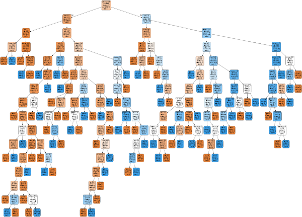
Classification Algorithms - Nave Bayes
Introduction to Nave Bayes Algorithm
Nave Bayes algorithms is a classification technique based on applying Bayes theorem with a strong assumption that all the predictors are independent to each other. In simple words, the assumption is that the presence of a feature in a class is independent to the presence of any other feature in the same class. For example, a phone may be considered as smart if it is having touch screen, internet facility, good camera etc. Though all these features are dependent on each other, they contribute independently to the probability of that the phone is a smart phone.
In Bayesian classification, the main interest is to find the posterior probabilities i.e. the probability of a label given some observed features, ( | ). With the help of Bayes theorem, we can express this in quantitative form as follows −
$P(L |features)= \frac{P(L)P(features |L)}{()}$Here, ( | ) is the posterior probability of class.
() is the prior probability of class.
( | ) is the likelihood which is the probability of predictor given class.
() is the prior probability of predictor.
Building model using Nave Bayes in Python
Python library, Scikit learn is the most useful library that helps us to build a Nave Bayes model in Python. We have the following three types of Nave Bayes model under Scikit learn Python library −
Gaussian Nave Bayes
It is the simplest Nave Bayes classifier having the assumption that the data from each label is drawn from a simple Gaussian distribution.
Multinomial Nave Bayes
Another useful Nave Bayes classifier is Multinomial Nave Bayes in which the features are assumed to be drawn from a simple Multinomial distribution. Such kind of Nave Bayes are most appropriate for the features that represents discrete counts.
Bernoulli Nave Bayes
Another important model is Bernoulli Nave Bayes in which features are assumed to be binary (0s and 1s). Text classification with bag of words model can be an application of Bernoulli Nave Bayes.
Example
Depending on our data set, we can choose any of the Nave Bayes model explained above. Here, we are implementing Gaussian Nave Bayes model in Python −
We will start with required imports as follows −
import numpy as np
import matplotlib.pyplot as plt
import seaborn as sns; sns.set()
Now, by using make_blobs() function of Scikit learn, we can generate blobs of points with Gaussian distribution as follows −
from sklearn.datasets import make_blobs
X, y = make_blobs(300, 2, centers=2, random_state=2, cluster_std=1.5)
plt.scatter(X[:, 0], X[:, 1], c=y, s=50, cmap='summer');
Next, for using GaussianNB model, we need to import and make its object as follows −
from sklearn.naive_bayes import GaussianNB
model_GBN = GaussianNB()
model_GNB.fit(X, y);
Now, we have to do prediction. It can be done after generating some new data as follows −
rng = np.random.RandomState(0)
Xnew = [-6, -14] + [14, 18] * rng.rand(2000, 2)
ynew = model_GNB.predict(Xnew)
Next, we are plotting new data to find its boundaries −
plt.scatter(X[:, 0], X[:, 1], c=y, s=50, cmap='summer')
lim = plt.axis()
plt.scatter(Xnew[:, 0], Xnew[:, 1], c=ynew, s=20, cmap='summer', alpha=0.1)
plt.axis(lim);
Now, with the help of following line of codes, we can find the posterior probabilities of first and second label −
yprob = model_GNB.predict_proba(Xnew)
yprob[-10:].round(3)
Output
array([[0.998, 0.002],
      [1. , 0. ],
      [0.987, 0.013],
      [1. , 0. ],
      [1. , 0. ],
      [1. , 0. ],
      [1. , 0. ],
      [1. , 0. ],
      [0. , 1. ],
      [0.986, 0.014]])
Pros & Cons
Pros
The followings are some pros of using Nave Bayes classifiers −
Nave Bayes classification is easy to implement and fast.
It will converge faster than discriminative models like logistic regression.
It requires less training data.
It is highly scalable in nature, or they scale linearly with the number of predictors and data points.
It can make probabilistic predictions and can handle continuous as well as discrete data.
Nave Bayes classification algorithm can be used for binary as well as multi-class classification problems both.
Cons
The followings are some cons of using Nave Bayes classifiers −
One of the most important cons of Nave Bayes classification is its strong feature independence because in real life it is almost impossible to have a set of features which are completely independent of each other.
Another issue with Nave Bayes classification is its zero frequency which means that if a categorial variable has a category but not being observed in training data set, then Nave Bayes model will assign a zero probability to it and it will be unable to make a prediction.
Applications of Nave Bayes classification
The following are some common applications of Nave Bayes classification −
Real-time prediction − Due to its ease of implementation and fast computation, it can be used to do prediction in real-time.
Multi-class prediction − Nave Bayes classification algorithm can be used to predict posterior probability of multiple classes of target variable.
Text classification − Due to the feature of multi-class prediction, Nave Bayes classification algorithms are well suited for text classification. That is why it is also used to solve problems like spam-filtering and sentiment analysis.
Recommendation system − Along with the algorithms like collaborative filtering, Nave Bayes makes a Recommendation system which can be used to filter unseen information and to predict weather a user would like the given resource or not.
Classification Algorithms - Random Forest
Introduction
Random forest is a supervised learning algorithm which is used for both classification as well as regression. But however, it is mainly used for classification problems. As we know that a forest is made up of trees and more trees means more robust forest. Similarly, random forest algorithm creates decision trees on data samples and then gets the prediction from each of them and finally selects the best solution by means of voting. It is an ensemble method which is better than a single decision tree because it reduces the over-fitting by averaging the result.
Working of Random Forest Algorithm
We can understand the working of Random Forest algorithm with the help of following steps −
Step1 − First, start with the selection of random samples from a given dataset.
Step2 − Next, this algorithm will construct a decision tree for every sample. Then it will get the prediction result from every decision tree.
Step3 − In this step, voting will be performed for every predicted result.
Step4 − At last, select the most voted prediction result as the final prediction result.
The following diagram will illustrate its working −
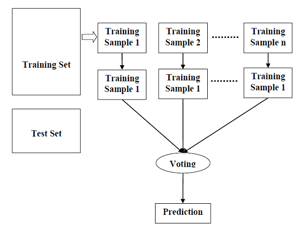
Implementation in Python
First, start with importing necessary Python packages −
import numpy as np
import matplotlib.pyplot as plt
import pandas as pd
Next, download the iris dataset from its weblink as follows −
path = "https://archive.ics.uci.edu/ml/machine-learning-databases/iris/iris.data"
Next, we need to assign column names to the dataset as follows −
headernames = ['sepal-length', 'sepal-width', 'petal-length', 'petal-width', 'Class']
Now, we need to read dataset to pandas dataframe as follows −
dataset = pd.read_csv(path, names=headernames)
dataset.head()
sepal-length |
sepal-width |
petal-length |
petal-width |
Class |
|
|---|---|---|---|---|---|
0 |
5.1 |
3.5 |
1.4 |
0.2 |
Iris-setosa |
1 |
4.9 |
3.0 |
1.4 |
0.2 |
Iris-setosa |
2 |
4.7 |
3.2 |
1.3 |
0.2 |
Iris-setosa |
3 |
4.6 |
3.1 |
1.5 |
0.2 |
Iris-setosa |
4 |
5.0 |
3.6 |
1.4 |
0.2 |
Iris-setosa |
Data Preprocessing will be done with the help of following script lines −
X = dataset.iloc[:, :-1].values
y = dataset.iloc[:, 4].values
Next, we will divide the data into train and test split. The following code will split the dataset into 70% training data and 30% of testing data −
from sklearn.model_selection import train_test_split
X_train, X_test, y_train, y_test = train_test_split(X, y, test_size=0.30)
Next, train the model with the help of RandomForestClassifier class of sklearn as follows −
from sklearn.ensemble import RandomForestClassifier
classifier = RandomForestClassifier(n_estimators=50)
classifier.fit(X_train, y_train)
At last, we need to make prediction. It can be done with the help of following script −
y_pred = classifier.predict(X_test)
Next, print the results as follows −
from sklearn.metrics import classification_report, confusion_matrix, accuracy_score
result = confusion_matrix(y_test, y_pred)
print("Confusion Matrix:")
print(result)
result1 = classification_report(y_test, y_pred)
print("Classification Report:",)
print (result1)
result2 = accuracy_score(y_test,y_pred)
print("Accuracy:",result2)
Output
Confusion Matrix:
[[14 0 0]
[ 0 18 1]
[ 0 0 12]]
Classification Report:
               precision       recall     f1-score       support
Iris-setosa        1.00         1.00        1.00         14
Iris-versicolor    1.00         0.95        0.97         19
Iris-virginica     0.92         1.00        0.96         12
micro avg          0.98         0.98        0.98         45
macro avg          0.97         0.98        0.98         45
weighted avg       0.98         0.98        0.98         45

Accuracy: 0.9777777777777777
Pros and Cons of Random Forest
Pros
The following are the advantages of Random Forest algorithm −
It overcomes the problem of overfitting by averaging or combining the results of different decision trees.
Random forests work well for a large range of data items than a single decision tree does.
Random forest has less variance then single decision tree.
Random forests are very flexible and possess very high accuracy.
Scaling of data does not require in random forest algorithm. It maintains good accuracy even after providing data without scaling.
Scaling of data does not require in random forest algorithm. It maintains good accuracy even after providing data without scaling.
Cons
The following are the disadvantages of Random Forest algorithm −
Complexity is the main disadvantage of Random forest algorithms.
Construction of Random forests are much harder and time-consuming than decision trees.
More computational resources are required to implement Random Forest algorithm.
It is less intuitive in case when we have a large collection of decision trees .
The prediction process using random forests is very time-consuming in comparison with other algorithms.
Regression Algorithms - Overview
Introduction to Regression
Regression is another important and broadly used statistical and machine learning tool. The key objective of regression-based tasks is to predict output labels or responses which are continues numeric values, for the given input data. The output will be based on what the model has learned in training phase. Basically, regression models use the input data features (independent variables) and their corresponding continuous numeric output values (dependent or outcome variables) to learn specific association between inputs and corresponding outputs.
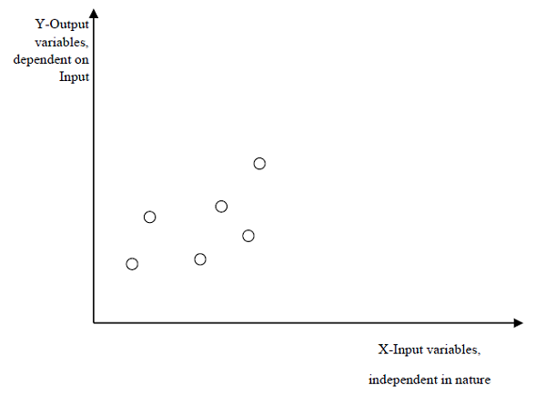
Types of Regression Models
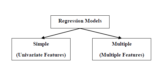
Regression models are of following two types −
Simple regression model − This is the most basic regression model in which predictions are formed from a single, univariate feature of the data.
Multiple regression model − As name implies, in this regression model the predictions are formed from multiple features of the data.
Building a Regressor in Python
Regressor model in Python can be constructed just like we constructed the classifier. Scikit-learn, a Python library for machine learning can also be used to build a regressor in Python.
In the following example, we will be building basic regression model that will fit a line to the data i.e. linear regressor. The necessary steps for building a regressor in Python are as follows −
Step1: Importing necessary python package
For building a regressor using scikit-learn, we need to import it along with other necessary packages. We can import the by using following script −
import numpy as np
from sklearn import linear_model
import sklearn.metrics as sm
import matplotlib.pyplot as plt
Step2: Importing dataset
After importing necessary package, we need a dataset to build regression prediction model. We can import it from sklearn dataset or can use other one as per our requirement. We are going to use our saved input data. We can import it with the help of following script −
input = r'C:\linear.txt'
Next, we need to load this data. We are using np.loadtxt function to load it.
input_data = np.loadtxt(input, delimiter=',')
X, y = input_data[:, :-1], input_data[:, -1]
Step3: Organizing data into training & testing sets
As we need to test our model on unseen data hence, we will divide our dataset into two parts: a training set and a test set. The following command will perform it −
training_samples = int(0.6 * len(X))
testing_samples = len(X) - num_training

X_train, y_train = X[:training_samples], y[:training_samples]

X_test, y_test = X[training_samples:], y[training_samples:]
Step4- Model evaluation & prediction
After dividing the data into training and testing we need to build the model. We will be using LineaRegression() function of Scikit-learn for this purpose. Following command will create a linear regressor object.
reg_linear= linear_model.LinearRegression()
Next, train this model with the training samples as follows −
reg_linear.fit(X_train, y_train)
Now, at last we need to do the prediction with the testing data.
y_test_pred = reg_linear.predict(X_test)
Step5- Plot & visualization
After prediction, we can plot and visualize it with the help of following script −
plt.scatter(X_test, y_test, color='red')
plt.plot(X_test, y_test_pred, color='black', linewidth=2)
plt.xticks(())
plt.yticks(())
plt.show()
Output
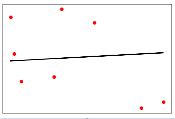
In the above output, we can see the regression line between the data points.
Step6- Performance computation − We can also compute the performance of our regression model with the help of various performance metrics as follows −
print("Regressor model performance:")
print("Mean absolute error(MAE) =", round(sm.mean_absolute_error(y_test, y_test_pred), 2))
print("Mean squared error(MSE) =", round(sm.mean_squared_error(y_test, y_test_pred), 2))
print("Median absolute error =", round(sm.median_absolute_error(y_test, y_test_pred), 2))
print("Explain variance score =", round(sm.explained_variance_score(y_test, y_test_pred), 2))
print("R2 score =", round(sm.r2_score(y_test, y_test_pred), 2))
Output
Regressor model performance:
Mean absolute error(MAE) = 1.78
Mean squared error(MSE) = 3.89
Median absolute error = 2.01
Explain variance score = -0.09
R2 score = -0.09
Types of ML Regression Algorithms
The most useful and popular ML regression algorithm is Linear regression algorithm which further divided into two types namely −
Simple Linear Regression algorithm
Multiple Linear Regression algorithm.
We will discuss about it and implement it in Python in the next chapter.
Applications
The applications of ML regression algorithms are as follows −
Forecasting or Predictive analysis − One of the important uses of regression is forecasting or predictive analysis. For example, we can forecast GDP, oil prices or in simple words the quantitative data that changes with the passage of time.
Optimization − We can optimize business processes with the help of regression. For example, a store manager can create a statistical model to understand the peek time of coming of customers.
Error correction − In business, taking correct decision is equally important as optimizing the business process. Regression can help us to take correct decision as well in correcting the already implemented decision.
Economics − It is the most used tool in economics. We can use regression to predict supply, demand, consumption, inventory investment etc.
Finance − A financial company is always interested in minimizing the risk portfolio and want to know the factors that affects the customers. All these can be predicted with the help of regression model.
Regression Algorithms - Linear Regression
Introduction to Linear Regression
Linear regression may be defined as the statistical model that analyzes the linear relationship between a dependent variable with given set of independent variables. Linear relationship between variables means that when the value of one or more independent variables will change (increase or decrease), the value of dependent variable will also change accordingly (increase or decrease).
Mathematically the relationship can be represented with the help of following equation −
Y = mX + b
Here, Y is the dependent variable we are trying to predict
X is the dependent variable we are using to make predictions.
m is the slop of the regression line which represents the effect X has on Y
b is a constant, known as the Y-intercept. If X = 0,Y would be equal to b.
Furthermore, the linear relationship can be positive or negative in nature as explained below −
Positive Linear Relationship
A linear relationship will be called positive if both independent and dependent variable increases. It can be understood with the help of following graph −
Negative Linear relationship
A linear relationship will be called positive if independent increases and dependent variable decreases. It can be understood with the help of following graph −
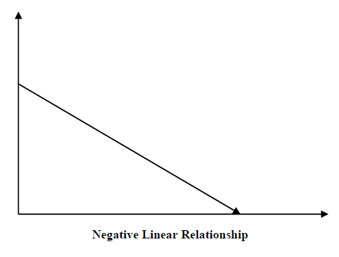
Types of Linear Regression
Linear regression is of the following two types −
Simple Linear Regression
Multiple Linear Regression
Simple Linear Regression (SLR)
It is the most basic version of linear regression which predicts a response using a single feature. The assumption in SLR is that the two variables are linearly related.
Python implementation
We can implement SLR in Python in two ways, one is to provide your own dataset and other is to use dataset from scikit-learn python library.
Example1 − In the following Python implementation example, we are using our own dataset.
First, we will start with importing necessary packages as follows −
%matplotlib inline
import numpy as np
import matplotlib.pyplot as plt
Next, define a function which will calculate the important values for SLR −
def coef_estimation(x, y):
The following script line will give number of observations n −
n = np.size(x)
The mean of x and y vector can be calculated as follows −
m_x, m_y = np.mean(x), np.mean(y)
We can find cross-deviation and deviation about x as follows −
SS_xy = np.sum(y*x) - n*m_y*m_x
SS_xx = np.sum(x*x) - n*m_x*m_x
Next, regression coefficients i.e. b can be calculated as follows −
b_1 = SS_xy / SS_xx
b_0 = m_y - b_1*m_x
return(b_0, b_1)
Next, we need to define a function which will plot the regression line as well as will predict the response vector −
def plot_regression_line(x, y, b):
The following script line will plot the actual points as scatter plot −
plt.scatter(x, y, color = "m", marker = "o", s = 30)
The following script line will predict response vector −
y_pred = b[0] + b[1]*x
The following script lines will plot the regression line and will put the labels on them −
plt.plot(x, y_pred, color = "g")
plt.xlabel('x')
plt.ylabel('y')
plt.show()
At last, we need to define main() function for providing dataset and calling the function we defined above −
def main():
   x = np.array([0, 1, 2, 3, 4, 5, 6, 7, 8, 9])
   y = np.array([100, 300, 350, 500, 750, 800, 850, 900, 1050, 1250])
   b = coef_estimation(x, y)
   print("Estimated coefficients:\nb_0 = {} \nb_1 = {}".format(b[0], b[1]))
   plot_regression_line(x, y, b)

if __name__ == "__main__":
main()
Output
Estimated coefficients:
b_0 = 154.5454545454545
b_1 = 117.87878787878788
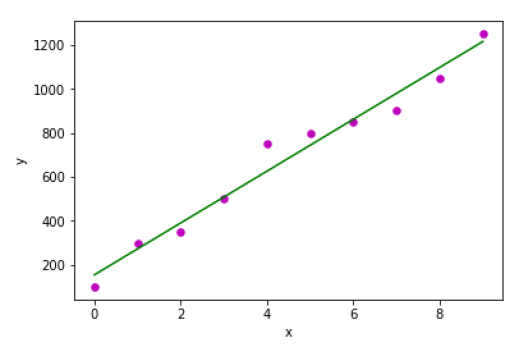
Example2 − In the following Python implementation example, we are using diabetes dataset from scikit-learn.
First, we will start with importing necessary packages as follows −
%matplotlib inline
import matplotlib.pyplot as plt
import numpy as np
from sklearn import datasets, linear_model
from sklearn.metrics import mean_squared_error, r2_score
Next, we will load the diabetes dataset and create its object −
diabetes = datasets.load_diabetes()
As we are implementing SLR, we will be using only one feature as follows −
X = diabetes.data[:, np.newaxis, 2]
Next, we need to split the data into training and testing sets as follows −
X_train = X[:-30]
X_test = X[-30:]
Next, we need to split the target into training and testing sets as follows −
y_train = diabetes.target[:-30]
y_test = diabetes.target[-30:]
Now, to train the model we need to create linear regression object as follows −
regr = linear_model.LinearRegression()
Next, train the model using the training sets as follows −
regr.fit(X_train, y_train)
Next, make predictions using the testing set as follows −
y_pred = regr.predict(X_test)
Next, we will be printing some coefficient like MSE, Variance score etc. as follows −
print('Coefficients: \n', regr.coef_)
print("Mean squared error: %.2f"
   % mean_squared_error(y_test, y_pred))
print('Variance score: %.2f' % r2_score(y_test, y_pred))
Now, plot the outputs as follows −
plt.scatter(X_test, y_test, color='blue')
plt.plot(X_test, y_pred, color='red', linewidth=3)
plt.xticks(())
plt.yticks(())
plt.show()
Output
Coefficients:
   [941.43097333]
Mean squared error: 3035.06
Variance score: 0.41
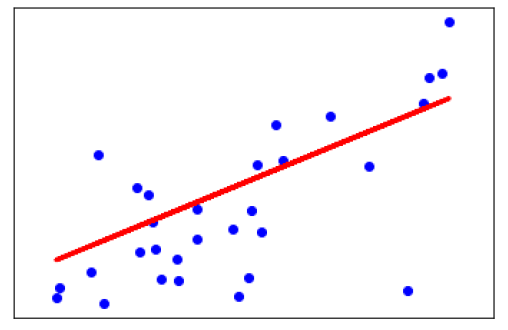
Multiple Linear Regression (MLR)
It is the extension of simple linear regression that predicts a response using two or more features. Mathematically we can explain it as follows −
Consider a dataset having n observations, p features i.e. independent variables and y as one response i.e. dependent variable the regression line for p features can be calculated as follows −
$h(x_{i})=b_{0}+b_{1}x_{i1}+b_{2}x_{i2}+...+b_{p}x_{ip}$Here, h(xi) is the predicted response value and b0,b1,b2,bp are the regression coefficients.
Multiple Linear Regression models always includes the errors in the data known as residual error which changes the calculation as follows −
$h(x_{i})=b_{0}+b_{1}x_{i1}+b_{2}x_{i2}+...+b_{p}x_{ip}+e_{i}$We can also write the above equation as follows −
$y_{i}=h(x_{i})+e_{i}$ or $e_{i}= y_{i} - h(x_{i})$Python Implementation
in this example, we will be using Boston housing dataset from scikit learn −
First, we will start with importing necessary packages as follows −
%matplotlib inline
import matplotlib.pyplot as plt
import numpy as np
from sklearn import datasets, linear_model, metrics
Next, load the dataset as follows −
boston = datasets.load_boston(return_X_y=False)
The following script lines will define feature matrix, X and response vector, Y −
X = boston.data
y = boston.target
Next, split the dataset into training and testing sets as follows −
from sklearn.model_selection import train_test_split
X_train, X_test, y_train, y_test = train_test_split(X, y, test_size=0.7, random_state=1)
Now, create linear regression object and train the model as follows −
reg = linear_model.LinearRegression()
reg.fit(X_train, y_train)
print('Coefficients: \n', reg.coef_)
print('Variance score: {}'.format(reg.score(X_test, y_test)))
plt.style.use('fivethirtyeight')
plt.scatter(reg.predict(X_train), reg.predict(X_train) - y_train,
      color = "green", s = 10, label = 'Train data')
plt.scatter(reg.predict(X_test), reg.predict(X_test) - y_test,
      color = "blue", s = 10, label = 'Test data')
plt.hlines(y = 0, xmin = 0, xmax = 50, linewidth = 2)
plt.legend(loc = 'upper right')
plt.title("Residual errors")
plt.show()
Output
Coefficients:
[-1.16358797e-01 6.44549228e-02 1.65416147e-01 1.45101654e+00
-1.77862563e+01 2.80392779e+00 4.61905315e-02 -1.13518865e+00
3.31725870e-01 -1.01196059e-02 -9.94812678e-01 9.18522056e-03
-7.92395217e-01]
Variance score: 0.709454060230326
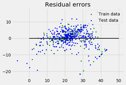
Assumptions
The following are some assumptions about dataset that is made by Linear Regression model −
Multi-collinearity − Linear regression model assumes that there is very little or no multi-collinearity in the data. Basically, multi-collinearity occurs when the independent variables or features have dependency in them.
Auto-correlation − Another assumption Linear regression model assumes is that there is very little or no auto-correlation in the data. Basically, auto-correlation occurs when there is dependency between residual errors.
Relationship between variables − Linear regression model assumes that the relationship between response and feature variables must be linear.
Clustering Algorithms - Overview
Introduction to Clustering
Clustering methods are one of the most useful unsupervised ML methods. These methods are used to find similarity as well as the relationship patterns among data samples and then cluster those samples into groups having similarity based on features.
Clustering is important because it determines the intrinsic grouping among the present unlabeled data. They basically make some assumptions about data points to constitute their similarity. Each assumption will construct different but equally valid clusters.
For example, below is the diagram which shows clustering system grouped together the similar kind of data in different clusters −
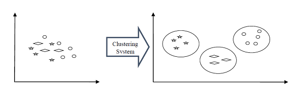
Cluster Formation Methods
It is not necessary that clusters will be formed in spherical form. Followings are some other cluster formation methods −
Density-based
In these methods, the clusters are formed as the dense region. The advantage of these methods is that they have good accuracy as well as good ability to merge two clusters. Ex. Density-Based Spatial Clustering of Applications with Noise (DBSCAN), Ordering Points to identify Clustering structure (OPTICS) etc.
Hierarchical-based
In these methods, the clusters are formed as a tree type structure based on the hierarchy. They have two categories namely, Agglomerative (Bottom up approach) and Divisive (Top down approach). Ex. Clustering using Representatives (CURE), Balanced iterative Reducing Clustering using Hierarchies (BIRCH) etc.
Partitioning
In these methods, the clusters are formed by portioning the objects into k clusters. Number of clusters will be equal to the number of partitions. Ex. K-means, Clustering Large Applications based upon randomized Search (CLARANS).
Grid
In these methods, the clusters are formed as a grid like structure. The advantage of these methods is that all the clustering operation done on these grids are fast and independent of the number of data objects. Ex. Statistical Information Grid (STING), Clustering in Quest (CLIQUE).
Measuring Clustering Performance
One of the most important consideration regarding ML model is assessing its performance or you can say models quality. In case of supervised learning algorithms, assessing the quality of our model is easy because we already have labels for every example.
On the other hand, in case of unsupervised learning algorithms we are not that much blessed because we deal with unlabeled data. But still we have some metrics that give the practitioner an insight about the happening of change in clusters depending on algorithm.
Before we deep dive into such metrics, we must understand that these metrics only evaluates the comparative performance of models against each other rather than measuring the validity of the models prediction. Followings are some of the metrics that we can deploy on clustering algorithms to measure the quality of model −
Silhouette Analysis
Silhouette analysis used to check the quality of clustering model by measuring the distance between the clusters. It basically provides us a way to assess the parameters like number of clusters with the help of Silhouette score. This score measures how close each point in one cluster is to points in the neighboring clusters.
Analysis of Silhouette Score
The range of Silhouette score is [-1, 1]. Its analysis is as follows −
+1 Score − Near +1 Silhouette score indicates that the sample is far away from its neighboring cluster.
0 Score − 0 Silhouette score indicates that the sample is on or very close to the decision boundary separating two neighboring clusters.
-1 Score &minusl -1 Silhouette score indicates that the samples have been assigned to the wrong clusters.
The calculation of Silhouette score can be done by using the following formula −
=()/ (,)
Here, = mean distance to the points in the nearest cluster
And, = mean intra-cluster distance to all the points.
Davis-Bouldin Index
DB index is another good metric to perform the analysis of clustering algorithms. With the help of DB index, we can understand the following points about clustering model −
Weather the clusters are well-spaced from each other or not?
How much dense the clusters are?
We can calculate DB index with the help of following formula −
$DB=\frac{1}{n}\displaystyle\sum\limits_{i=1}^n max_{j\neq{i}}\left(\frac{\sigma_{i}+\sigma_{j}}{d(c_{i},c_{j})}\right)$Here, = number of clusters
σi = average distance of all points in cluster from the cluster centroid .
Less the DB index, better the clustering model is.
Dunn Index
It works same as DB index but there are following points in which both differs −
The Dunn index considers only the worst case i.e. the clusters that are close together while DB index considers dispersion and separation of all the clusters in clustering model.
Dunn index increases as the performance increases while DB index gets better when clusters are well-spaced and dense.
We can calculate Dunn index with the help of following formula −
$D=\frac{min_{1\leq i <{j}\leq{n}}P(i,j)}{mix_{1\leq i < k \leq n}q(k)}$Here, ,, = each indices for clusters
= inter-cluster distance
q = intra-cluster distance
Types of ML Clustering Algorithms
The following are the most important and useful ML clustering algorithms −
K-means Clustering
This clustering algorithm computes the centroids and iterates until we it finds optimal centroid. It assumes that the number of clusters are already known. It is also called flat clustering algorithm. The number of clusters identified from data by algorithm is represented by K in K-means.
Mean-Shift Algorithm
It is another powerful clustering algorithm used in unsupervised learning. Unlike K-means clustering, it does not make any assumptions hence it is a non-parametric algorithm.
Hierarchical Clustering
It is another unsupervised learning algorithm that is used to group together the unlabeled data points having similar characteristics.
We will be discussing all these algorithms in detail in the upcoming chapters.
Applications of Clustering
We can find clustering useful in the following areas −
Data summarization and compression − Clustering is widely used in the areas where we require data summarization, compression and reduction as well. The examples are image processing and vector quantization.
Collaborative systems and customer segmentation − Since clustering can be used to find similar products or same kind of users, it can be used in the area of collaborative systems and customer segmentation.
Serve as a key intermediate step for other data mining tasks − Cluster analysis can generate a compact summary of data for classification, testing, hypothesis generation; hence, it serves as a key intermediate step for other data mining tasks also.
Trend detection in dynamic data − Clustering can also be used for trend detection in dynamic data by making various clusters of similar trends.
Social network analysis − Clustering can be used in social network analysis. The examples are generating sequences in images, videos or audios.
Biological data analysis − Clustering can also be used to make clusters of images, videos hence it can successfully be used in biological data analysis.
Clustering Algorithms - K-means Algorithm
Introduction to K-Means Algorithm
K-means clustering algorithm computes the centroids and iterates until we it finds optimal centroid. It assumes that the number of clusters are already known. It is also called flat clustering algorithm. The number of clusters identified from data by algorithm is represented by K in K-means.
In this algorithm, the data points are assigned to a cluster in such a manner that the sum of the squared distance between the data points and centroid would be minimum. It is to be understood that less variation within the clusters will lead to more similar data points within same cluster.
Working of K-Means Algorithm
We can understand the working of K-Means clustering algorithm with the help of following steps −
Step1 − First, we need to specify the number of clusters, K, need to be generated by this algorithm.
Step2 − Next, randomly select K data points and assign each data point to a cluster. In simple words, classify the data based on the number of data points.
Step3 − Now it will compute the cluster centroids.
Step4 − Next, keep iterating the following until we find optimal centroid which is the assignment of data points to the clusters that are not changing any more −
4.1 − First, the sum of squared distance between data points and centroids would be computed.
4.2 − Now, we have to assign each data point to the cluster that is closer than other cluster (centroid).
4.3 − At last compute the centroids for the clusters by taking the average of all data points of that cluster.
K-means follows Expectation-Maximization approach to solve the problem. The Expectation-step is used for assigning the data points to the closest cluster and the Maximization-step is used for computing the centroid of each cluster.
While working with K-means algorithm we need to take care of the following things −
While working with clustering algorithms including K-Means, it is recommended to standardize the data because such algorithms use distance-based measurement to determine the similarity between data points.
Due to the iterative nature of K-Means and random initialization of centroids, K-Means may stick in a local optimum and may not converge to global optimum. That is why it is recommended to use different initializations of centroids.
Implementation in Python
The following two examples of implementing K-Means clustering algorithm will help us in its better understanding −
Example1
It is a simple example to understand how k-means works. In this example, we are going to first generate 2D dataset containing 4 different blobs and after that will apply k-means algorithm to see the result.
First, we will start by importing the necessary packages −
%matplotlib inline
import matplotlib.pyplot as plt
import seaborn as sns; sns.set()
import numpy as np
from sklearn.cluster import KMeans
The following code will generate the 2D, containing four blobs −
from sklearn.datasets.samples_generator import make_blobs
X, y_true = make_blobs(n_samples=400, centers=4, cluster_std=0.60, random_state=0)
Next, the following code will help us to visualize the dataset −
plt.scatter(X[:, 0], X[:, 1], s=20);
plt.show()
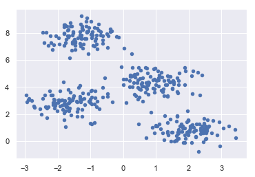
Next, make an object of KMeans along with providing number of clusters, train the model and do the prediction as follows −
kmeans = KMeans(n_clusters=4)
kmeans.fit(X)
y_kmeans = kmeans.predict(X)
Now, with the help of following code we can plot and visualize the clusters centers picked by k-means Python estimator −
plt.scatter(X[:, 0], X[:, 1], c=y_kmeans, s=20, cmap='summer')
centers = kmeans.cluster_centers_
plt.scatter(centers[:, 0], centers[:, 1], c='blue', s=100, alpha=0.9);
plt.show()

Example 2
Let us move to another example in which we are going to apply K-means clustering on simple digits dataset. K-means will try to identify similar digits without using the original label information.
First, we will start by importing the necessary packages −
%matplotlib inline
import matplotlib.pyplot as plt
import seaborn as sns; sns.set()
import numpy as np
from sklearn.cluster import KMeans
Next, load the digit dataset from sklearn and make an object of it. We can also find number of rows and columns in this dataset as follows −
from sklearn.datasets import load_digits
digits = load_digits()
digits.data.shape
Output
(1797, 64)
The above output shows that this dataset is having 1797 samples with 64 features.
We can perform the clustering as we did in Example 1 above −
kmeans = KMeans(n_clusters=10, random_state=0)
clusters = kmeans.fit_predict(digits.data)
kmeans.cluster_centers_.shape
Output
(10, 64)
The above output shows that K-means created 10 clusters with 64 features.
fig, ax = plt.subplots(2, 5, figsize=(8, 3))
centers = kmeans.cluster_centers_.reshape(10, 8, 8)
for axi, center in zip(ax.flat, centers):
   axi.set(xticks=[], yticks=[])
   axi.imshow(center, interpolation='nearest', cmap=plt.cm.binary)
Output
As output, we will get following image showing clusters centers learned by k-means.
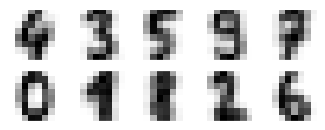
The following lines of code will match the learned cluster labels with the true labels found in them −
from scipy.stats import mode
labels = np.zeros_like(clusters)
for i in range(10):
   mask = (clusters == i)
   labels[mask] = mode(digits.target[mask])[0]
Next, we can check the accuracy as follows −
from sklearn.metrics import accuracy_score
accuracy_score(digits.target, labels)
Output
0.7935447968836951
The above output shows that the accuracy is around 80%.
Advantages and Disadvantages
Advantages
The following are some advantages of K-Means clustering algorithms −
It is very easy to understand and implement.
If we have large number of variables then, K-means would be faster than Hierarchical clustering.
On re-computation of centroids, an instance can change the cluster.
Tighter clusters are formed with K-means as compared to Hierarchical clustering.
Disadvantages
The following are some disadvantages of K-Means clustering algorithms −
It is a bit difficult to predict the number of clusters i.e. the value of k.
Output is strongly impacted by initial inputs like number of clusters (value of k).
Order of data will have strong impact on the final output.
It is very sensitive to rescaling. If we will rescale our data by means of normalization or standardization, then the output will completely change.final output.
It is not good in doing clustering job if the clusters have a complicated geometric shape.
Applications of K-Means Clustering Algorithm
The main goals of cluster analysis are −
To get a meaningful intuition from the data we are working with.
Cluster-then-predict where different models will be built for different subgroups.
To fulfill the above-mentioned goals, K-means clustering is performing well enough. It can be used in following applications −
Market segmentation
Document Clustering
Image segmentation
Image compression
Customer segmentation
Analyzing the trend on dynamic data
Clustering Algorithms - Mean Shift Algorithm
Introduction to Mean-Shift Algorithm
As discussed earlier, it is another powerful clustering algorithm used in unsupervised learning. Unlike K-means clustering, it does not make any assumptions; hence it is a non-parametric algorithm.
Mean-shift algorithm basically assigns the datapoints to the clusters iteratively by shifting points towards the highest density of datapoints i.e. cluster centroid.
The difference between K-Means algorithm and Mean-Shift is that later one does not need to specify the number of clusters in advance because the number of clusters will be determined by the algorithm w.r.t data.
Working of Mean-Shift Algorithm
We can understand the working of Mean-Shift clustering algorithm with the help of following steps −
Step1 − First, start with the data points assigned to a cluster of their own.
Step2 − Next, this algorithm will compute the centroids.
Step3 − In this step, location of new centroids will be updated.
Step4 − Now, the process will be iterated and moved to the higher density region.
Step5 − At last, it will be stopped once the centroids reach at position from where it cannot move further.
Implementation in Python
It is a simple example to understand how Mean-Shift algorithm works. In this example, we are going to first generate 2D dataset containing 4 different blobs and after that will apply Mean-Shift algorithm to see the result.
%matplotlib inline
import numpy as np
from sklearn.cluster import MeanShift
import matplotlib.pyplot as plt
from matplotlib import style
style.use("ggplot")
from sklearn.datasets.samples_generator import make_blobs
centers = [[3,3,3],[4,5,5],[3,10,10]]
X, _ = make_blobs(n_samples = 700, centers = centers, cluster_std = 0.5)
plt.scatter(X[:,0],X[:,1])
plt.show()
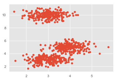
ms = MeanShift()
ms.fit(X)
labels = ms.labels_
cluster_centers = ms.cluster_centers_
print(cluster_centers)
n_clusters_ = len(np.unique(labels))
print("Estimated clusters:", n_clusters_)
colors = 10*['r.','g.','b.','c.','k.','y.','m.']
for i in range(len(X)):
   plt.plot(X[i][0], X[i][1], colors[labels[i]], markersize = 3)
plt.scatter(cluster_centers[:,0],cluster_centers[:,1],
      marker=".",color='k', s=20, linewidths = 5, zorder=10)
plt.show()
Output
[[ 2.98462798 9.9733794 10.02629344]
[ 3.94758484 4.99122771 4.99349433]
[ 3.00788996 3.03851268 2.99183033]]
Estimated clusters: 3
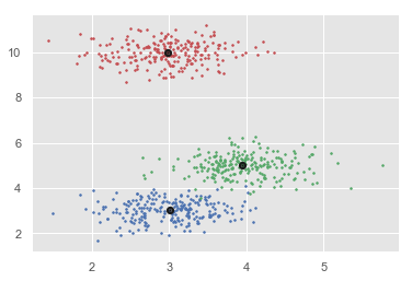
Advantages and Disadvantages
Advantages
The following are some advantages of Mean-Shift clustering algorithm −
It does not need to make any model assumption as like in K-means or Gaussian mixture.
It can also model the complex clusters which have nonconvex shape.
It only needs one parameter named bandwidth which automatically determines the number of clusters.
There is no issue of local minima as like in K-means.
No problem generated from outliers.
Disadvantages
The following are some disadvantages of Mean-Shift clustering algorithm −
Mean-shift algorithm does not work well in case of high dimension, where number of clusters changes abruptly.
We do not have any direct control on the number of clusters but in some applications, we need a specific number of clusters.
It cannot differentiate between meaningful and meaningless modes.
Clustering Algorithms - Hierarchical Clustering
Introduction to Hierarchical Clustering
Hierarchical clustering is another unsupervised learning algorithm that is used to group together the unlabeled data points having similar characteristics. Hierarchical clustering algorithms falls into following two categories −
Agglomerative hierarchical algorithms − In agglomerative hierarchical algorithms, each data point is treated as a single cluster and then successively merge or agglomerate (bottom-up approach) the pairs of clusters. The hierarchy of the clusters is represented as a dendrogram or tree structure.
Divisive hierarchical algorithms − On the other hand, in divisive hierarchical algorithms, all the data points are treated as one big cluster and the process of clustering involves dividing (Top-down approach) the one big cluster into various small clusters.
Steps to Perform Agglomerative Hierarchical Clustering
We are going to explain the most used and important Hierarchical clustering i.e. agglomerative. The steps to perform the same is as follows −
Step1 − Treat each data point as single cluster. Hence, we will be having, say K clusters at start. The number of data points will also be K at start.
Step2 − Now, in this step we need to form a big cluster by joining two closet datapoints. This will result in total of K-1 clusters.
Step3 − Now, to form more clusters we need to join two closet clusters. This will result in total of K-2 clusters.
Step4 − Now, to form one big cluster repeat the above three steps until K would become 0 i.e. no more data points left to join.
Step5 − At last, after making one single big cluster, dendrograms will be used to divide into multiple clusters depending upon the problem.
Role of Dendrograms in Agglomerative Hierarchical Clustering
As we discussed in the last step, the role of dendrogram starts once the big cluster is formed. Dendrogram will be used to split the clusters into multiple cluster of related data points depending upon our problem. It can be understood with the help of following example −
Example1
To understand, let us start with importing the required libraries as follows −
%matplotlib inline
import matplotlib.pyplot as plt
import numpy as np
Next, we will be plotting the datapoints we have taken for this example −
X = np.array([[7,8],[12,20],[17,19],[26,15],[32,37],[87,75],[73,85], [62,80],[73,60],[87,96],])
labels = range(1, 11)
plt.figure(figsize=(10, 7))
plt.subplots_adjust(bottom=0.1)
plt.scatter(X[:,0],X[:,1], label='True Position')
for label, x, y in zip(labels, X[:, 0], X[:, 1]):
   plt.annotate(label,xy=(x, y), xytext=(-3, 3),textcoords='offset points', ha='right', va='bottom')
plt.show()
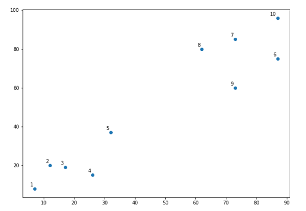
From the above diagram, it is very easy to see that we have two clusters in out datapoints but in the real world data, there can be thousands of clusters. Next, we will be plotting the dendrograms of our datapoints by using Scipy library −
from scipy.cluster.hierarchy import dendrogram, linkage
from matplotlib import pyplot as plt
linked = linkage(X, 'single')
labelList = range(1, 11)
plt.figure(figsize=(10, 7))
dendrogram(linked, orientation='top',labels=labelList, distance_sort='descending',show_leaf_counts=True)
plt.show()
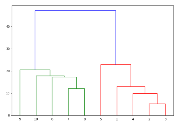
Now, once the big cluster is formed, the longest vertical distance is selected. A vertical line is then drawn through it as shown in the following diagram. As the horizontal line crosses the blue line at two points, the number of clusters would be two.
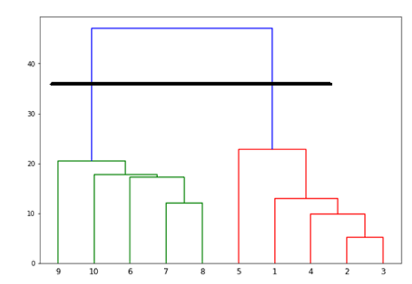
Next, we need to import the class for clustering and call its fit_predict method to predict the cluster. We are importing AgglomerativeClustering class of sklearn.cluster library −
from sklearn.cluster import AgglomerativeClustering
cluster = AgglomerativeClustering(n_clusters=2, affinity='euclidean', linkage='ward')
cluster.fit_predict(X)
Next, plot the cluster with the help of following code −
plt.scatter(X[:,0],X[:,1], c=cluster.labels_, cmap='rainbow')
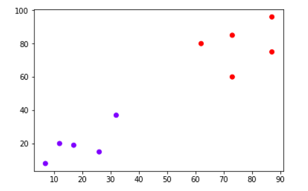
The above diagram shows the two clusters from our datapoints.
Example2
As we understood the concept of dendrograms from the simple example discussed above, let us move to another example in which we are creating clusters of the data point in Pima Indian Diabetes Dataset by using hierarchical clustering −
import matplotlib.pyplot as plt
import pandas as pd
%matplotlib inline
import numpy as np
from pandas import read_csv
path = r"C:\pima-indians-diabetes.csv"
headernames = ['preg', 'plas', 'pres', 'skin', 'test', 'mass', 'pedi', 'age', 'class']
data = read_csv(path, names=headernames)
array = data.values
X = array[:,0:8]
Y = array[:,8]
data.shape
(768, 9)
data.head()
| slno. | preg | Plas | Pres | skin | test | mass | pedi | age | class |
|---|---|---|---|---|---|---|---|---|---|
| 0 | 6 | 148 | 72 | 35 | 0 | 33.6 | 0.627 | 50 | 1 |
| 1 | 1 | 85 | 66 | 29 | 0 | 26.6 | 0.351 | 31 | 0 |
| 2 | 8 | 183 | 64 | 0 | 0 | 23.3 | 0.672 | 32 | 1 |
| 3 | 1 | 89 | 66 | 23 | 94 | 28.1 | 0.167 | 21 | 0 |
| 4 | 0 | 137 | 40 | 35 | 168 | 43.1 | 2.288 | 33 | 1 |
patient_data = data.iloc[:, 3:5].values
import scipy.cluster.hierarchy as shc
plt.figure(figsize=(10, 7))
plt.title("Patient Dendograms")
dend = shc.dendrogram(shc.linkage(data, method='ward'))
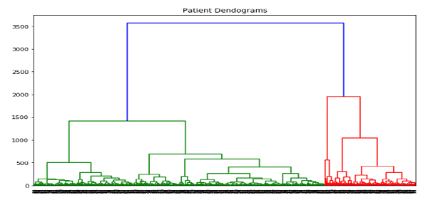
from sklearn.cluster import AgglomerativeClustering
cluster = AgglomerativeClustering(n_clusters=4, affinity='euclidean', linkage='ward')
cluster.fit_predict(patient_data)
plt.figure(figsize=(10, 7))
plt.scatter(patient_data[:,0], patient_data[:,1], c=cluster.labels_, cmap='rainbow')
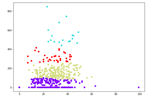
KNN Algorithm - Finding Nearest Neighbors
Introduction
K-nearest neighbors (KNN) algorithm is a type of supervised ML algorithm which can be used for both classification as well as regression predictive problems. However, it is mainly used for classification predictive problems in industry. The following two properties would define KNN well −
Lazy learning algorithm − KNN is a lazy learning algorithm because it does not have a specialized training phase and uses all the data for training while classification.
Non-parametric learning algorithm − KNN is also a non-parametric learning algorithm because it doesnt assume anything about the underlying data.
Working of KNN Algorithm
K-nearest neighbors (KNN) algorithm uses feature similarity to predict the values of new datapoints which further means that the new data point will be assigned a value based on how closely it matches the points in the training set. We can understand its working with the help of following steps −
Step1 − For implementing any algorithm, we need dataset. So during the first step of KNN, we must load the training as well as test data.
Step2 − Next, we need to choose the value of K i.e. the nearest data points. K can be any integer.
Step3 − For each point in the test data do the following −
3.1 − Calculate the distance between test data and each row of training data with the help of any of the method namely: Euclidean, Manhattan or Hamming distance. The most commonly used method to calculate distance is Euclidean.
3.2 − Now, based on the distance value, sort them in ascending order.
3.3 − Next, it will choose the top K rows from the sorted array.
3.4 − Now, it will assign a class to the test point based on most frequent class of these rows.
Step4 − End
Example
The following is an example to understand the concept of K and working of KNN algorithm −
Suppose we have a dataset which can be plotted as follows −
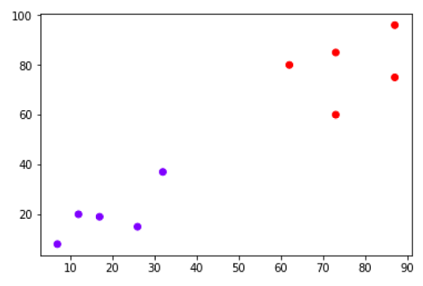
Now, we need to classify new data point with black dot (at point 60,60) into blue or red class. We are assuming K = 3 i.e. it would find three nearest data points. It is shown in the next diagram −
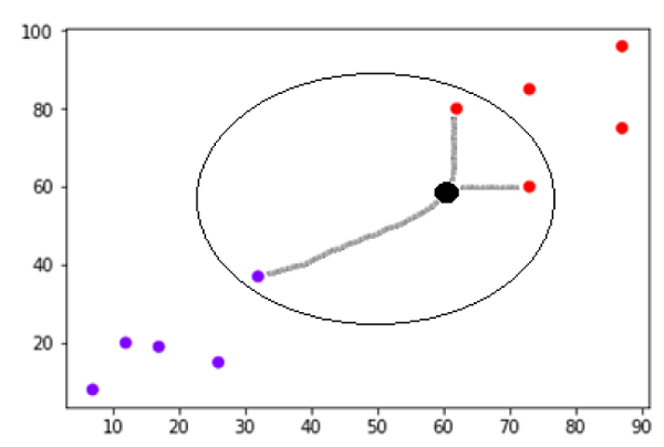
We can see in the above diagram the three nearest neighbors of the data point with black dot. Among those three, two of them lies in Red class hence the black dot will also be assigned in red class.
Implementation in Python
As we know K-nearest neighbors (KNN) algorithm can be used for both classification as well as regression. The following are the recipes in Python to use KNN as classifier as well as regressor −
KNN as Classifier
First, start with importing necessary python packages −
import numpy as np
import matplotlib.pyplot as plt
import pandas as pd
Next, download the iris dataset from its weblink as follows −
path = "https://archive.ics.uci.edu/ml/machine-learning-databases/iris/iris.data"
Next, we need to assign column names to the dataset as follows −
headernames = ['sepal-length', 'sepal-width', 'petal-length', 'petal-width', 'Class']
Now, we need to read dataset to pandas dataframe as follows −
dataset = pd.read_csv(path, names=headernames)
dataset.head()
| slno. | sepal-length | sepal-width | petal-length | petal-width | Class |
|---|---|---|---|---|---|
| 0 | 5.1 | 3.5 | 1.4 | 0.2 | Iris-setosa |
| 1 | 4.9 | 3.0 | 1.4 | 0.2 | Iris-setosa |
| 2 | 4.7 | 3.2 | 1.3 | 0.2 | Iris-setosa |
| 3 | 4.6 | 3.1 | 1.5 | 0.2 | Iris-setosa |
| 4 | 5.0 | 3.6 | 1.4 | 0.2 | Iris-setosa |
Data Preprocessing will be done with the help of following script lines −
X = dataset.iloc[:, :-1].values
y = dataset.iloc[:, 4].values
Next, we will divide the data into train and test split. Following code will split the dataset into 60% training data and 40% of testing data −
from sklearn.model_selection import train_test_split
X_train, X_test, y_train, y_test = train_test_split(X, y, test_size=0.40)
Next, data scaling will be done as follows −
from sklearn.preprocessing import StandardScaler
scaler = StandardScaler()
scaler.fit(X_train)
X_train = scaler.transform(X_train)
X_test = scaler.transform(X_test)
Next, train the model with the help of KNeighborsClassifier class of sklearn as follows −
from sklearn.neighbors import KNeighborsClassifier
classifier = KNeighborsClassifier(n_neighbors=8)
classifier.fit(X_train, y_train)
At last we need to make prediction. It can be done with the help of following script −
y_pred = classifier.predict(X_test)
Next, print the results as follows −
from sklearn.metrics import classification_report, confusion_matrix, accuracy_score
result = confusion_matrix(y_test, y_pred)
print("Confusion Matrix:")
print(result)
result1 = classification_report(y_test, y_pred)
print("Classification Report:",)
print (result1)
result2 = accuracy_score(y_test,y_pred)
print("Accuracy:",result2)
Output
Confusion Matrix:
[[21 0 0]
[ 0 16 0]
[ 0 7 16]]
Classification Report:
            precision      recall       f1-score       support
Iris-setosa       1.00        1.00         1.00          21
Iris-versicolor   0.70        1.00         0.82          16
Iris-virginica    1.00        0.70         0.82          23
micro avg         0.88        0.88         0.88          60
macro avg         0.90        0.90         0.88          60
weighted avg      0.92        0.88         0.88          60


Accuracy: 0.8833333333333333
KNN as Regressor
First, start with importing necessary Python packages −
import numpy as np
import pandas as pd
Next, download the iris dataset from its weblink as follows −
path = "https://archive.ics.uci.edu/ml/machine-learning-databases/iris/iris.data"
Next, we need to assign column names to the dataset as follows −
headernames = ['sepal-length', 'sepal-width', 'petal-length', 'petal-width', 'Class']
Now, we need to read dataset to pandas dataframe as follows −
data = pd.read_csv(url, names=headernames)
array = data.values
X = array[:,:2]
Y = array[:,2]
data.shape

output:(150, 5)
Next, import KNeighborsRegressor from sklearn to fit the model −
from sklearn.neighbors import KNeighborsRegressor
knnr = KNeighborsRegressor(n_neighbors=10)
knnr.fit(X, y)
At last, we can find the MSE as follows −
print ("The MSE is:",format(np.power(y-knnr.predict(X),2).mean()))
Output
The MSE is: 0.12226666666666669
Pros and Cons of KNN
Pros
It is very simple algorithm to understand and interpret.
It is very useful for nonlinear data because there is no assumption about data in this algorithm.
It is a versatile algorithm as we can use it for classification as well as regression.
It has relatively high accuracy but there are much better supervised learning models than KNN.
Cons
It is computationally a bit expensive algorithm because it stores all the training data.
High memory storage required as compared to other supervised learning algorithms.
Prediction is slow in case of big N.
It is very sensitive to the scale of data as well as irrelevant features.
Applications of KNN
The following are some of the areas in which KNN can be applied successfully −
Banking System
KNN can be used in banking system to predict weather an individual is fit for loan approval? Does that individual have the characteristics similar to the defaulters one?
Calculating Credit Ratings
KNN algorithms can be used to find an individuals credit rating by comparing with the persons having similar traits.
Politics
With the help of KNN algorithms, we can classify a potential voter into various classes like Will Vote, Will not Vote, Will Vote to Party Congress, Will Vote to Party BJP.
Other areas in which KNN algorithm can be used are Speech Recognition, Handwriting Detection, Image Recognition and Video Recognition.
Machine Learning - Performance Metrics
There are various metrics which we can use to evaluate the performance of ML algorithms, classification as well as regression algorithms. We must carefully choose the metrics for evaluating ML performance because −
How the performance of ML algorithms is measured and compared will be dependent entirely on the metric you choose.
How you weight the importance of various characteristics in the result will be influenced completely by the metric you choose.
Performance Metrics for Classification Problems
We have discussed classification and its algorithms in the previous chapters. Here, we are going to discuss various performance metrics that can be used to evaluate predictions for classification problems.
Confusion Matrix
It is the easiest way to measure the performance of a classification problem where the output can be of two or more type of classes. A confusion matrix is nothing but a table with two dimensions viz. Actual and Predicted and furthermore, both the dimensions have True Positives (TP), True Negatives (TN), False Positives (FP), False Negatives (FN) as shown below −
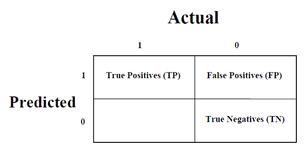
Explanation of the terms associated with confusion matrix are as follows −
True Positives (TP) − It is the case when both actual class & predicted class of data point is 1.
True Negatives (TN) − It is the case when both actual class & predicted class of data point is 0.
False Positives (FP) − It is the case when actual class of data point is 0 & predicted class of data point is 1.
False Negatives (FN) − It is the case when actual class of data point is 1 & predicted class of data point is 0.
We can use confusion_matrix function of sklearn.metrics to compute Confusion Matrix of our classification model.
Classification Accuracy
It is most common performance metric for classification algorithms. It may be defined as the number of correct predictions made as a ratio of all predictions made. We can easily calculate it by confusion matrix with the help of following formula −
$Accuracy =\frac{TP+TN}{+++}$We can use accuracy_score function of sklearn.metrics to compute accuracy of our classification model.
Classification Report
This report consists of the scores of Precisions, Recall, F1 and Support. They are explained as follows −
Precision
Precision, used in document retrievals, may be defined as the number of correct documents returned by our ML model. We can easily calculate it by confusion matrix with the help of following formula −
$Precision=\frac{TP}{TP+FP}$Recall or Sensitivity
Recall may be defined as the number of positives returned by our ML model. We can easily calculate it by confusion matrix with the help of following formula −
$Recall =\frac{TP}{TP+FN}$Specificity
Specificity, in contrast to recall, may be defined as the number of negatives returned by our ML model. We can easily calculate it by confusion matrix with the help of following formula −
$Specificity =\frac{TN}{TN+FP}$Support
Support may be defined as the number of samples of the true response that lies in each class of target values.
F1 Score
This score will give us the harmonic mean of precision and recall. Mathematically, F1 score is the weighted average of the precision and recall. The best value of F1 would be 1 and worst would be 0. We can calculate F1 score with the help of following formula −
= ( ) / ( + )
F1 score is having equal relative contribution of precision and recall.
We can use classification_report function of sklearn.metrics to get the classification report of our classification model.
AUC (Area Under ROC curve)
AUC (Area Under Curve)-ROC (Receiver Operating Characteristic) is a performance metric, based on varying threshold values, for classification problems. As name suggests, ROC is a probability curve and AUC measure the separability. In simple words, AUC-ROC metric will tell us about the capability of model in distinguishing the classes. Higher the AUC, better the model.
Mathematically, it can be created by plotting TPR (True Positive Rate) i.e. Sensitivity or recall vs FPR (False Positive Rate) i.e. 1-Specificity, at various threshold values. Following is the graph showing ROC, AUC having TPR at y-axis and FPR at x-axis −

We can use roc_auc_score function of sklearn.metrics to compute AUC-ROC.
LOGLOSS (Logarithmic Loss)
It is also called Logistic regression loss or cross-entropy loss. It basically defined on probability estimates and measures the performance of a classification model where the input is a probability value between 0 and 1. It can be understood more clearly by differentiating it with accuracy. As we know that accuracy is the count of predictions (predicted value = actual value) in our model whereas Log Loss is the amount of uncertainty of our prediction based on how much it varies from the actual label. With the help of Log Loss value, we can have more accurate view of the performance of our model. We can use log_loss function of sklearn.metrics to compute Log Loss.
Example
The following is a simple recipe in Python which will give us an insight about how we can use the above explained performance metrics on binary classification model −
from sklearn.metrics import confusion_matrix
from sklearn.metrics import accuracy_score
from sklearn.metrics import classification_report
from sklearn.metrics import roc_auc_score
from sklearn.metrics import log_loss
X_actual = [1, 1, 0, 1, 0, 0, 1, 0, 0, 0]
Y_predic = [1, 0, 1, 1, 1, 0, 1, 1, 0, 0]
results = confusion_matrix(X_actual, Y_predic)
print ('Confusion Matrix :')
print(results)
print ('Accuracy Score is',accuracy_score(X_actual, Y_predic))
print ('Classification Report : ')
print (classification_report(X_actual, Y_predic))
print('AUC-ROC:',roc_auc_score(X_actual, Y_predic))
print('LOGLOSS Value is',log_loss(X_actual, Y_predic))
Output
Confusion Matrix :
[[3 3]
[1 3]]
Accuracy Score is 0.6
Classification Report :
            precision      recall      f1-score       support
      0       0.75          0.50      0.60           6
      1       0.50          0.75      0.60           4
micro avg     0.60          0.60      0.60           10
macro avg     0.62          0.62      0.60           10
weighted avg  0.65          0.60      0.60           10
AUC-ROC:  0.625
LOGLOSS Value is 13.815750437193334
Performance Metrics for Regression Problems
We have discussed regression and its algorithms in previous chapters. Here, we are going to discuss various performance metrics that can be used to evaluate predictions for regression problems.
Mean Absolute Error (MAE)
It is the simplest error metric used in regression problems. It is basically the sum of average of the absolute difference between the predicted and actual values. In simple words, with MAE, we can get an idea of how wrong the predictions were. MAE does not indicate the direction of the model i.e. no indication about underperformance or overperformance of the model. The following is the formula to calculate MAE −
$MAE = \frac{1}{n}\sum|Y -\hat{Y}|$Here, =Actual Output Values
And $\hat{Y}$= Predicted Output Values.
We can use mean_absolute_error function of sklearn.metrics to compute MAE.
Mean Square Error (MSE)
MSE is like the MAE, but the only difference is that the it squares the difference of actual and predicted output values before summing them all instead of using the absolute value. The difference can be noticed in the following equation −
$MSE = \frac{1}{n}\sum(Y -\hat{Y})$Here, =Actual Output Values
And $\hat{Y}$ = Predicted Output Values.
We can use mean_squared_error function of sklearn.metrics to compute MSE.
R Squared (R2)
R Squared metric is generally used for explanatory purpose and provides an indication of the goodness or fit of a set of predicted output values to the actual output values. The following formula will help us understanding it −
$R^{2} = 1 -\frac{\frac{1}{n}\sum_{i{=1}}^n(Y_{i}-\hat{Y_{i}})^2}{\frac{1}{n}\sum_{i{=1}}^n(Y_{i}-\bar{Y_i)^2}}$In the above equation, numerator is MSE and the denominator is the variance in values.
We can use r2_score function of sklearn.metrics to compute R squared value.
Example
The following is a simple recipe in Python which will give us an insight about how we can use the above explained performance metrics on regression model −
from sklearn.metrics import r2_score
from sklearn.metrics import mean_absolute_error
from sklearn.metrics import mean_squared_error
X_actual = [5, -1, 2, 10]
Y_predic = [3.5, -0.9, 2, 9.9]
print ('R Squared =',r2_score(X_actual, Y_predic))
print ('MAE =',mean_absolute_error(X_actual, Y_predic))
print ('MSE =',mean_squared_error(X_actual, Y_predic))
Output
R Squared = 0.9656060606060606
MAE = 0.42499999999999993
MSE = 0.5674999999999999
Machine Learning - Automatic Workflows
Introduction
In order to execute and produce results successfully, a machine learning model must automate some standard workflows. The process of automate these standard workflows can be done with the help of Scikit-learn Pipelines. From a data scientists perspective, pipeline is a generalized, but very important concept. It basically allows data flow from its raw format to some useful information. The working of pipelines can be understood with the help of following diagram −
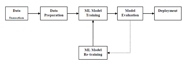
The blocks of ML pipelines are as follows −
Data ingestion − As the name suggests, it is the process of importing the data for use in ML project. The data can be extracted in real time or batches from single or multiple systems. It is one of the most challenging steps because the quality of data can affect the whole ML model.
Data Preparation − After importing the data, we need to prepare data to be used for our ML model. Data preprocessing is one of the most important technique of data preparation.
ML Model Training − Next step is to train our ML model. We have various ML algorithms like supervised, unsupervised, reinforcement to extract the features from data, and make predictions.
Model Evaluation − Next, we need to evaluate the ML model. In case of AutoML pipeline, ML model can be evaluated with the help of various statistical methods and business rules.
ML Model retraining − In case of AutoML pipeline, it is not necessary that the first model is best one. The first model is considered as a baseline model and we can train it repeatably to increase models accuracy.
Deployment − At last, we need to deploy the model. This step involves applying and migrating the model to business operations for their use.
Challenges Accompanying ML Pipelines
In order to create ML pipelines, data scientists face many challenges. These challenges fall into the following three categories −
Quality of Data
The success of any ML model depends heavily on the quality of data. If the data we are providing to ML model is not accurate, reliable and robust, then we are going to end with wrong or misleading output.
Data Reliability
Another challenge associated with ML pipelines is the reliability of data we are providing to the ML model. As we know, there can be various sources from which data scientist can acquire data but to get the best results, it must be assured that the data sources are reliable and trusted.
Data Accessibility
To get the best results out of ML pipelines, the data itself must be accessible which requires consolidation, cleansing and curation of data. As a result of data accessibility property, metadata will be updated with new tags.
Modelling ML Pipeline and Data Preparation
Data leakage, happening from training dataset to testing dataset, is an important issue for data scientist to deal with while preparing data for ML model. Generally, at the time of data preparation, data scientist uses techniques like standardization or normalization on entire dataset before learning. But these techniques cannot help us from the leakage of data because the training dataset would have been influenced by the scale of the data in the testing dataset.
By using ML pipelines, we can prevent this data leakage because pipelines ensure that data preparation like standardization is constrained to each fold of our cross-validation procedure.
Example
The following is an example in Python that demonstrate data preparation and model evaluation workflow. For this purpose, we are using Pima Indian Diabetes dataset from Sklearn. First, we will be creating pipeline that standardized the data. Then a Linear Discriminative analysis model will be created and at last the pipeline will be evaluated using 10-fold cross validation.
First, import the required packages as follows −
from pandas import read_csv
from sklearn.model_selection import KFold
from sklearn.model_selection import cross_val_score
from sklearn.preprocessing import StandardScaler
from sklearn.pipeline import Pipeline
from sklearn.discriminant_analysis import LinearDiscriminantAnalysis
Now, we need to load the Pima diabetes dataset as did in previous examples −
path = r"C:\pima-indians-diabetes.csv"
headernames = ['preg', 'plas', 'pres', 'skin', 'test', 'mass', 'pedi', 'age', 'class']
data = read_csv(path, names=headernames)
array = data.values
Next, we will create a pipeline with the help of the following code −
estimators = []
estimators.append(('standardize', StandardScaler()))
estimators.append(('lda', LinearDiscriminantAnalysis()))
model = Pipeline(estimators)
At last, we are going to evaluate this pipeline and output its accuracy as follows −
kfold = KFold(n_splits=20, random_state=7)
results = cross_val_score(model, X, Y, cv=kfold)
print(results.mean())
Output
0.7790148448043184
The above output is the summary of accuracy of the setup on the dataset.
Modelling ML Pipeline and Feature Extraction
Data leakage can also happen at feature extraction step of ML model. That is why feature extraction procedures should also be restricted to stop data leakage in our training dataset. As in the case of data preparation, by using ML pipelines, we can prevent this data leakage also. FeatureUnion, a tool provided by ML pipelines can be used for this purpose.
Example
The following is an example in Python that demonstrates feature extraction and model evaluation workflow. For this purpose, we are using Pima Indian Diabetes dataset from Sklearn.
First, 3 features will be extracted with PCA (Principal Component Analysis). Then, 6 features will be extracted with Statistical Analysis. After feature extraction, result of multiple feature selection and extraction procedures will be combined by using
FeatureUnion tool. At last, a Logistic Regression model will be created, and the pipeline will be evaluated using 10-fold cross validation.
First, import the required packages as follows −
from pandas import read_csv
from sklearn.model_selection import KFold
from sklearn.model_selection import cross_val_score
from sklearn.pipeline import Pipeline
from sklearn.pipeline import FeatureUnion
from sklearn.linear_model import LogisticRegression
from sklearn.decomposition import PCA
from sklearn.feature_selection import SelectKBest
Now, we need to load the Pima diabetes dataset as did in previous examples −
path = r"C:\pima-indians-diabetes.csv"
headernames = ['preg', 'plas', 'pres', 'skin', 'test', 'mass', 'pedi', 'age', 'class']
data = read_csv(path, names=headernames)
array = data.values
Next, feature union will be created as follows −
features = []
features.append(('pca', PCA(n_components=3)))
features.append(('select_best', SelectKBest(k=6)))
feature_union = FeatureUnion(features)
Next, pipeline will be creating with the help of following script lines −
estimators = []
estimators.append(('feature_union', feature_union))
estimators.append(('logistic', LogisticRegression()))
model = Pipeline(estimators)
At last, we are going to evaluate this pipeline and output its accuracy as follows −
kfold = KFold(n_splits=20, random_state=7)
results = cross_val_score(model, X, Y, cv=kfold)
print(results.mean())
Output
0.7789811066126855
The above output is the summary of accuracy of the setup on the dataset.
Improving Performance of ML Models
Performance Improvement with Ensembles
Ensembles can give us boost in the machine learning result by combining several models. Basically, ensemble models consist of several individually trained supervised learning models and their results are merged in various ways to achieve better predictive performance compared to a single model. Ensemble methods can be divided into following two groups −
Sequential ensemble methods
As the name implies, in these kind of ensemble methods, the base learners are generated sequentially. The motivation of such methods is to exploit the dependency among base learners.
Parallel ensemble methods
As the name implies, in these kind of ensemble methods, the base learners are generated in parallel. The motivation of such methods is to exploit the independence among base learners.
Ensemble Learning Methods
The following are the most popular ensemble learning methods i.e. the methods for combining the predictions from different models −
Bagging
The term bagging is also known as bootstrap aggregation. In bagging methods, ensemble model tries to improve prediction accuracy and decrease model variance by combining predictions of individual models trained over randomly generated training samples. The final prediction of ensemble model will be given by calculating the average of all predictions from the individual estimators. One of the best examples of bagging methods are random forests.
Boosting
In boosting method, the main principle of building ensemble model is to build it incrementally by training each base model estimator sequentially. As the name suggests, it basically combine several week base learners, trained sequentially over multiple iterations of training data, to build powerful ensemble. During the training of week base learners, higher weights are assigned to those learners which were misclassified earlier. The example of boosting method is AdaBoost.
Voting
In this ensemble learning model, multiple models of different types are built and some simple statistics, like calculating mean or median etc., are used to combine the predictions. This prediction will serve as the additional input for training to make the final prediction.
Bagging Ensemble Algorithms
The following are three bagging ensemble algorithms −
Bagged Decision Tree
As we know that bagging ensemble methods work well with the algorithms that have high variance and, in this concern, the best one is decision tree algorithm. In the following Python recipe, we are going to build bagged decision tree ensemble model by using BaggingClassifier function of sklearn with DecisionTreeClasifier (a classification & regression trees algorithm) on Pima Indians diabetes dataset.
First, import the required packages as follows −
from pandas import read_csv
from sklearn.model_selection import KFold
from sklearn.model_selection import cross_val_score
from sklearn.ensemble import BaggingClassifier
from sklearn.tree import DecisionTreeClassifier
Now, we need to load the Pima diabetes dataset as we did in the previous examples −
path = r"C:\pima-indians-diabetes.csv"
headernames = ['preg', 'plas', 'pres', 'skin', 'test', 'mass', 'pedi', 'age', 'class']
data = read_csv(path, names=headernames)
array = data.values
X = array[:,0:8]
Y = array[:,8]
Next, give the input for 10-fold cross validation as follows −
seed = 7
kfold = KFold(n_splits=10, random_state=seed)
cart = DecisionTreeClassifier()
We need to provide the number of trees we are going to build. Here we are building 150 trees −
num_trees = 150
Next, build the model with the help of following script −
model = BaggingClassifier(base_estimator=cart, n_estimators=num_trees, random_state=seed)
Calculate and print the result as follows −
results = cross_val_score(model, X, Y, cv=kfold)
print(results.mean())
Output
0.7733766233766234
The output above shows that we got around 77% accuracy of our bagged decision tree classifier model.
Random Forest
It is an extension of bagged decision trees. For individual classifiers, the samples of training dataset are taken with replacement, but the trees are constructed in such a way that reduces the correlation between them. Also, a random subset of features is considered to choose each split point rather than greedily choosing the best split point in construction of each tree.
In the following Python recipe, we are going to build bagged random forest ensemble model by using RandomForestClassifier class of sklearn on Pima Indians diabetes dataset.
First, import the required packages as follows −
from pandas import read_csv
from sklearn.model_selection import KFold
from sklearn.model_selection import cross_val_score
from sklearn.ensemble import RandomForestClassifier
Now, we need to load the Pima diabetes dataset as did in previous examples −
path = r"C:\pima-indians-diabetes.csv"
headernames = ['preg', 'plas', 'pres', 'skin', 'test', 'mass', 'pedi', 'age', 'class']
data = read_csv(path, names=headernames)
array = data.values
X = array[:,0:8]
Y = array[:,8]
Next, give the input for 10-fold cross validation as follows −
seed = 7
kfold = KFold(n_splits=10, random_state=seed)
We need to provide the number of trees we are going to build. Here we are building 150 trees with split points chosen from 5 features −
num_trees = 150
max_features = 5
Next, build the model with the help of following script −
model = RandomForestClassifier(n_estimators=num_trees, max_features=max_features)
Calculate and print the result as follows −
results = cross_val_score(model, X, Y, cv=kfold)
print(results.mean())
Output
0.7629357484620642
The output above shows that we got around 76% accuracy of our bagged random forest classifier model.
Extra Trees
It is another extension of bagged decision tree ensemble method. In this method, the random trees are constructed from the samples of the training dataset.
In the following Python recipe, we are going to build extra tree ensemble model by using ExtraTreesClassifier class of sklearn on Pima Indians diabetes dataset.
First, import the required packages as follows −
from pandas import read_csv from sklearn.model_selection import KFold from sklearn.model_selection import cross_val_score from sklearn.ensemble import ExtraTreesClassifier
Now, we need to load the Pima diabetes dataset as did in previous examples −
path = r"C:\pima-indians-diabetes.csv" headernames = ['preg', 'plas', 'pres', 'skin', 'test', 'mass', 'pedi', 'age', 'class'] data = read_csv(path, names=headernames) array = data.values X = array[:,0:8] Y = array[:,8]
Next, give the input for 10-fold cross validation as follows −
seed = 7 kfold = KFold(n_splits=10, random_state=seed)
We need to provide the number of trees we are going to build. Here we are building 150 trees with split points chosen from 5 features −
num_trees = 150 max_features = 5
Next, build the model with the help of following script −
model = ExtraTreesClassifier(n_estimators=num_trees, max_features=max_features)
Calculate and print the result as follows −
results = cross_val_score(model, X, Y, cv=kfold) print(results.mean())
Output
0.7551435406698566
The output above shows that we got around 75.5% accuracy of our bagged extra trees classifier model.
Boosting Ensemble Algorithms
The followings are the two most common boosting ensemble algorithms −
AdaBoost
It is one the most successful boosting ensemble algorithm. The main key of this algorithm is in the way they give weights to the instances in dataset. Due to this the algorithm needs to pay less attention to the instances while constructing subsequent models.
In the following Python recipe, we are going to build Ada Boost ensemble model for classification by using AdaBoostClassifier class of sklearn on Pima Indians diabetes dataset.
First, import the required packages as follows −
from pandas import read_csv from sklearn.model_selection import KFold from sklearn.model_selection import cross_val_score from sklearn.ensemble import AdaBoostClassifier
Now, we need to load the Pima diabetes dataset as did in previous examples −
path = r"C:\pima-indians-diabetes.csv" headernames = ['preg', 'plas', 'pres', 'skin', 'test', 'mass', 'pedi', 'age', 'class'] data = read_csv(path, names=headernames) array = data.values X = array[:,0:8] Y = array[:,8]
Next, give the input for 10-fold cross validation as follows −
seed = 5 kfold = KFold(n_splits=10, random_state=seed)
We need to provide the number of trees we are going to build. Here we are building 150 trees with split points chosen from 5 features −
num_trees = 50
Next, build the model with the help of following script −
model = AdaBoostClassifier(n_estimators=num_trees, random_state=seed)
Calculate and print the result as follows −
results = cross_val_score(model, X, Y, cv=kfold) print(results.mean())
Output
0.7539473684210527
The output above shows that we got around 75% accuracy of our AdaBoost classifier ensemble model.
Stochastic Gradient Boosting
It is also called Gradient Boosting Machines. In the following Python recipe, we are going to build Stochastic Gradient Boostingensemble model for classification by using GradientBoostingClassifier class of sklearn on Pima Indians diabetes dataset.
First, import the required packages as follows −
from pandas import read_csv from sklearn.model_selection import KFold from sklearn.model_selection import cross_val_score from sklearn.ensemble import GradientBoostingClassifier
Now, we need to load the Pima diabetes dataset as did in previous examples −
path = r"C:\pima-indians-diabetes.csv" headernames = ['preg', 'plas', 'pres', 'skin', 'test', 'mass', 'pedi', 'age', 'class'] data = read_csv(path, names=headernames) array = data.values X = array[:,0:8] Y = array[:,8]
Next, give the input for 10-fold cross validation as follows −
seed = 5 kfold = KFold(n_splits=10, random_state=seed)
We need to provide the number of trees we are going to build. Here we are building 150 trees with split points chosen from 5 features −
num_trees = 50
Next, build the model with the help of following script −
model = GradientBoostingClassifier(n_estimators=num_trees, random_state=seed)
Calculate and print the result as follows −
results = cross_val_score(model, X, Y, cv=kfold) print(results.mean())
Output
0.7746582365003418
The output above shows that we got around 77.5% accuracy of our Gradient Boosting classifier ensemble model.
Voting Ensemble Algorithms
As discussed, voting first creates two or more standalone models from training dataset and then a voting classifier will wrap the model along with taking the average of the predictions of sub-model whenever needed new data.
In the following Python recipe, we are going to build Voting ensemble model for classification by using VotingClassifier class of sklearn on Pima Indians diabetes dataset. We are combining the predictions of logistic regression, Decision Tree classifier and SVM together for a classification problem as follows −
First, import the required packages as follows −
from pandas import read_csv from sklearn.model_selection import KFold from sklearn.model_selection import cross_val_score from sklearn.linear_model import LogisticRegression from sklearn.tree import DecisionTreeClassifier from sklearn.svm import SVC from sklearn.ensemble import VotingClassifier
Now, we need to load the Pima diabetes dataset as did in previous examples −
path = r"C:\pima-indians-diabetes.csv" headernames = ['preg', 'plas', 'pres', 'skin', 'test', 'mass', 'pedi', 'age', 'class'] data = read_csv(path, names=headernames) array = data.values X = array[:,0:8] Y = array[:,8]
Next, give the input for 10-fold cross validation as follows −
kfold = KFold(n_splits=10, random_state=7)
Next, we need to create sub-models as follows −
estimators = []
model1 = LogisticRegression()
estimators.append(('logistic', model1))
model2 = DecisionTreeClassifier()
estimators.append(('cart', model2))
model3 = SVC()
estimators.append(('svm', model3))
Now, create the voting ensemble model by combining the predictions of above created sub models.
ensemble = VotingClassifier(estimators) results = cross_val_score(ensemble, X, Y, cv=kfold) print(results.mean())
Output
0.7382262474367738
The output above shows that we got around 74% accuracy of our voting classifier ensemble model.
Improving Performance of ML Model (Contd)
Performance Improvement with Algorithm Tuning
As we know that ML models are parameterized in such a way that their behavior can be adjusted for a specific problem. Algorithm tuning means finding the best combination of these parameters so that the performance of ML model can be improved. This process sometimes called hyperparameter optimization and the parameters of algorithm itself are called hyperparameters and coefficients found by ML algorithm are called parameters.
Here, we are going to discuss about some methods for algorithm parameter tuning provided by Python Scikit-learn.
Grid Search Parameter Tuning
It is a parameter tuning approach. The key point of working of this method is that it builds and evaluate the model methodically for every possible combination of algorithm parameter specified in a grid. Hence, we can say that this algorithm is having search nature.
Example
In the following Python recipe, we are going to perform grid search by using GridSearchCV class of sklearn for evaluating various alpha values for the Ridge Regression algorithm on Pima Indians diabetes dataset.
First, import the required packages as follows −
import numpy from pandas import read_csv from sklearn.linear_model import Ridge from sklearn.model_selection import GridSearchCV
Now, we need to load the Pima diabetes dataset as did in previous examples −
path = r"C:\pima-indians-diabetes.csv" headernames = ['preg', 'plas', 'pres', 'skin', 'test', 'mass', 'pedi', 'age', 'class'] data = read_csv(path, names=headernames) array = data.values X = array[:,0:8] Y = array[:,8]
Next, evaluate the various alpha values as follows −
alphas = numpy.array([1,0.1,0.01,0.001,0.0001,0]) param_grid = dict(alpha=alphas)
Now, we need to apply grid search on our model −
model = Ridge() grid = GridSearchCV(estimator=model, param_grid=param_grid) grid.fit(X, Y)
Print the result with following script line −
print(grid.best_score_) print(grid.best_estimator_.alpha)
Output
0.2796175593129722 1.0
The above output gives us the optimal score and the set of parameters in the grid that achieved that score. The alpha value in this case is 1.0.
Random Search Parameter Tuning
It is a parameter tuning approach. The key point of working of this method is that it samples the algorithm parameters from a random distribution for a fixed number of iterations.
Example
In the following Python recipe, we are going to perform random search by using RandomizedSearchCV class of sklearn for evaluating different alpha values between 0 and 1 for the Ridge Regression algorithm on Pima Indians diabetes dataset.
First, import the required packages as follows −
import numpy from pandas import read_csv from scipy.stats import uniform from sklearn.linear_model import Ridge from sklearn.model_selection import RandomizedSearchCV
Now, we need to load the Pima diabetes dataset as did in previous examples −
path = r"C:\pima-indians-diabetes.csv" headernames = ['preg', 'plas', 'pres', 'skin', 'test', 'mass', 'pedi', 'age', 'class'] data = read_csv(path, names=headernames) array = data.values X = array[:,0:8] Y = array[:,8]
Next, evaluate the various alpha values on Ridge regression algorithm as follows −
param_grid = {'alpha': uniform()}
model = Ridge()
random_search = RandomizedSearchCV(estimator=model, param_distributions=param_grid, n_iter=50,
random_state=7)
random_search.fit(X, Y)
Print the result with following script line −
print(random_search.best_score_) print(random_search.best_estimator_.alpha)
Output
0.27961712703051084 0.9779895119966027 0.9779895119966027
The above output gives us the optimal score just similar to the grid search.
