- ML - Home
- ML - Introduction
- ML - Getting Started
- ML - Basic Concepts
- ML - Ecosystem
- ML - Python Libraries
- ML - Applications
- ML - Life Cycle
- ML - Required Skills
- ML - Implementation
- ML - Challenges & Common Issues
- ML - Limitations
- ML - Reallife Examples
- ML - Data Structure
- ML - Mathematics
- ML - Artificial Intelligence
- ML - Neural Networks
- ML - Deep Learning
- ML - Getting Datasets
- ML - Categorical Data
- ML - Data Loading
- ML - Data Understanding
- ML - Data Preparation
- ML - Models
- ML - Supervised Learning
- ML - Unsupervised Learning
- ML - Semi-supervised Learning
- ML - Reinforcement Learning
- ML - Supervised vs. Unsupervised
- Machine Learning Data Visualization
- ML - Data Visualization
- ML - Histograms
- ML - Density Plots
- ML - Box and Whisker Plots
- ML - Correlation Matrix Plots
- ML - Scatter Matrix Plots
- Statistics for Machine Learning
- ML - Statistics
- ML - Mean, Median, Mode
- ML - Standard Deviation
- ML - Percentiles
- ML - Data Distribution
- ML - Skewness and Kurtosis
- ML - Bias and Variance
- ML - Hypothesis
- Regression Analysis In ML
- ML - Regression Analysis
- ML - Linear Regression
- ML - Simple Linear Regression
- ML - Multiple Linear Regression
- ML - Polynomial Regression
- Classification Algorithms In ML
- ML - Classification Algorithms
- ML - Logistic Regression
- ML - K-Nearest Neighbors (KNN)
- ML - Naïve Bayes Algorithm
- ML - Decision Tree Algorithm
- ML - Support Vector Machine
- ML - Random Forest
- ML - Confusion Matrix
- ML - Stochastic Gradient Descent
- Clustering Algorithms In ML
- ML - Clustering Algorithms
- ML - Centroid-Based Clustering
- ML - K-Means Clustering
- ML - K-Medoids Clustering
- ML - Mean-Shift Clustering
- ML - Hierarchical Clustering
- ML - Density-Based Clustering
- ML - DBSCAN Clustering
- ML - OPTICS Clustering
- ML - HDBSCAN Clustering
- ML - BIRCH Clustering
- ML - Affinity Propagation
- ML - Distribution-Based Clustering
- ML - Agglomerative Clustering
- Dimensionality Reduction In ML
- ML - Dimensionality Reduction
- ML - Feature Selection
- ML - Feature Extraction
- ML - Backward Elimination
- ML - Forward Feature Construction
- ML - High Correlation Filter
- ML - Low Variance Filter
- ML - Missing Values Ratio
- ML - Principal Component Analysis
- Reinforcement Learning
- ML - Reinforcement Learning Algorithms
- ML - Exploitation & Exploration
- ML - Q-Learning
- ML - REINFORCE Algorithm
- ML - SARSA Reinforcement Learning
- ML - Actor-critic Method
- ML - Monte Carlo Methods
- ML - Temporal Difference
- Deep Reinforcement Learning
- ML - Deep Reinforcement Learning
- ML - Deep Reinforcement Learning Algorithms
- ML - Deep Q-Networks
- ML - Deep Deterministic Policy Gradient
- ML - Trust Region Methods
- Quantum Machine Learning
- ML - Quantum Machine Learning
- ML - Quantum Machine Learning with Python
- Machine Learning Miscellaneous
- ML - Performance Metrics
- ML - Automatic Workflows
- ML - Boost Model Performance
- ML - Gradient Boosting
- ML - Bootstrap Aggregation (Bagging)
- ML - Cross Validation
- ML - AUC-ROC Curve
- ML - Grid Search
- ML - Data Scaling
- ML - Train and Test
- ML - Association Rules
- ML - Apriori Algorithm
- ML - Gaussian Discriminant Analysis
- ML - Cost Function
- ML - Bayes Theorem
- ML - Precision and Recall
- ML - Adversarial
- ML - Stacking
- ML - Epoch
- ML - Perceptron
- ML - Regularization
- ML - Overfitting
- ML - P-value
- ML - Entropy
- ML - MLOps
- ML - Data Leakage
- ML - Monetizing Machine Learning
- ML - Types of Data
- Machine Learning - Resources
- ML - Quick Guide
- ML - Cheatsheet
- ML - Interview Questions
- ML - Useful Resources
- ML - Discussion
Logistic Regression in Machine Learning
Introduction to Logistic Regression
Logistic regression is a supervised learning classification algorithm used to predict the probability of a target variable. The nature of target or dependent variable is dichotomous, which means there would be only two possible classes.
In simple words, the dependent variable is binary in nature having data coded as either 1 (stands for success/yes) or 0 (stands for failure/no).
Mathematically, a logistic regression model predicts P(Y=1) as a function of X. It is one of the simplest ML algorithms that can be used for various classification problems such as spam detection, Diabetes prediction, cancer detection etc.
Types of Logistic Regression
Generally, logistic regression means binary logistic regression having binary target variables, but there can be two more categories of target variables that can be predicted by it. Based on those number of categories, Logistic regression can be divided into following types −
Binary or Binomial
In such a kind of classification, a dependent variable will have only two possible types either 1 and 0. For example, these variables may represent success or failure, yes or no, win or loss etc.
Multinomial
In such a kind of classification, dependent variable can have 3 or more possible unordered types or the types having no quantitative significance. For example, these variables may represent "Type A" or "Type B" or "Type C".
Ordinal
In such a kind of classification, dependent variable can have 3 or more possible ordered types or the types having a quantitative significance. For example, these variables may represent "poor" or "good", "very good", "Excellent" and each category can have the scores like 0,1,2,3.
Logistic Regression Assumptions
Before diving into the implementation of logistic regression, we must be aware of the following assumptions about the same −
In case of binary logistic regression, the target variables must be binary always and the desired outcome is represented by the factor level 1.
There should not be any multi-collinearity in the model, which means the independent variables must be independent of each other .
We must include meaningful variables in our model.
We should choose a large sample size for logistic regression.
Binary Logistic Regression Model
The simplest form of logistic regression is binary or binomial logistic regression in which the target or dependent variable can have only 2 possible types either 1 or 0. It allows us to model a relationship between multiple predictor variables and a binary/binomial target variable. In case of logistic regression, the linear function is basically used as an input to another function such as in the following relation −
$$h_{\theta}{(x)}=g(\theta^{T}x) 0h_{\theta}1$$Here, is the logistic or sigmoid function which can be given as follows −
$$g(z)= \frac{1}{1+e^{-z}} =\theta ^{T}$$To sigmoid curve can be represented with the help of following graph. We can see the values of y-axis lie between 0 and 1 and crosses the axis at 0.5.
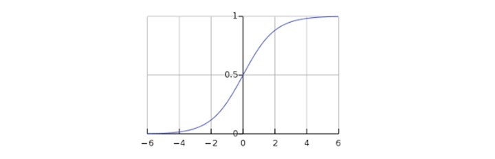
The classes can be divided into positive or negative. The output comes under the probability of positive class if it lies between 0 and 1. For our implementation, we are interpreting the output of hypothesis function as positive if it is 0.5, otherwise negative.
We also need to define a loss function to measure how well the algorithm performs using the weights on functions, represented by theta as follows −
$$=()$$
$$J(\theta) = \frac{1}{m}.(-y^{T}log(h) - (1 -y)^Tlog(1-h))$$
Now, after defining the loss function our prime goal is to minimize the loss function. It can be done with the help of fitting the weights which means by increasing or decreasing the weights. With the help of derivatives of the loss function w.r.t each weight, we would be able to know what parameters should have high weight and what should have smaller weight.
The following gradient descent equation tells us how loss would change if we modified the parameters −
$$\frac{()}{\theta_{j}}=\frac{1}{m}X^{T}(())$$Implementation of Binary Logistic Regression Model in Python
Now we will implement the above concept of binomial logistic regression in Python. For this purpose, we are using a multivariate flower dataset named iris which have 3 classes of 50 instances each, but we will be using the first two feature columns. Every class represents a type of iris flower.
First, we need to import the necessary libraries as follows −
import numpy as np
import matplotlib.pyplot as plt
import seaborn as sns
from sklearn import datasets
Next, load the iris dataset as follows −
iris = datasets.load_iris()
X = iris.data[:, :2]
y = (iris.target != 0) * 1
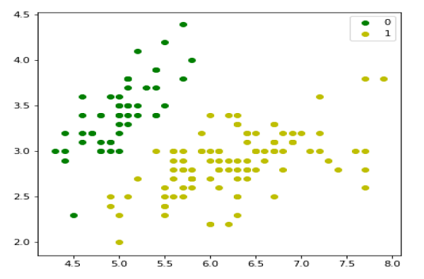
We can plot our training data s follows −
plt.figure(figsize=(6, 6))
plt.scatter(X[y == 0][:, 0], X[y == 0][:, 1], color='g', label='0')
plt.scatter(X[y == 1][:, 0], X[y == 1][:, 1], color='y', label='1')
plt.legend();
Next, we will define sigmoid function, loss function and gradient descend as follows −
class LogisticRegression:
   def __init__(self, lr=0.01, num_iter=100000, fit_intercept=True, verbose=False):
      self.lr = lr
      self.num_iter = num_iter
      self.fit_intercept = fit_intercept
      self.verbose = verbose
   def __add_intercept(self, X):
      intercept = np.ones((X.shape[0], 1))
      return np.concatenate((intercept, X), axis=1)
   def __sigmoid(self, z):
      return 1 / (1 + np.exp(-z))
   def __loss(self, h, y):
      return (-y * np.log(h) - (1 - y) * np.log(1 - h)).mean()
   def fit(self, X, y):
      if self.fit_intercept:
         X = self.__add_intercept(X)
Now, initialize the weights as follows −
self.theta = np.zeros(X.shape[1])
   for i in range(self.num_iter):
      z = np.dot(X, self.theta)
      h = self.__sigmoid(z)
      gradient = np.dot(X.T, (h - y)) / y.size
      self.theta -= self.lr * gradient
      z = np.dot(X, self.theta)
      h = self.__sigmoid(z)
      loss = self.__loss(h, y)
      if(self.verbose ==True and i % 10000 == 0):
         print(f'loss: {loss} \t')
With the help of the following script, we can predict the output probabilities −
def predict_prob(self, X):
   if self.fit_intercept:
      X = self.__add_intercept(X)
   return self.__sigmoid(np.dot(X, self.theta))
def predict(self, X):
   return self.predict_prob(X).round()
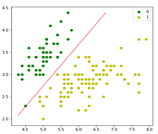
Next, we can evaluate the model and plot it as follows −
model = LogisticRegression(lr=0.1, num_iter=300000)
preds = model.predict(X)
(preds == y).mean()

plt.figure(figsize=(10, 6))
plt.scatter(X[y == 0][:, 0], X[y == 0][:, 1], color='g', label='0')
plt.scatter(X[y == 1][:, 0], X[y == 1][:, 1], color='y', label='1')
plt.legend()
x1_min, x1_max = X[:,0].min(), X[:,0].max(),
x2_min, x2_max = X[:,1].min(), X[:,1].max(),
xx1, xx2 = np.meshgrid(np.linspace(x1_min, x1_max), np.linspace(x2_min, x2_max))
grid = np.c_[xx1.ravel(), xx2.ravel()]
probs = model.predict_prob(grid).reshape(xx1.shape)
plt.contour(xx1, xx2, probs, [0.5], linewidths=1, colors='red');
Multinomial Logistic Regression Model
Another useful form of logistic regression is multinomial logistic regression in which the target or dependent variable can have 3 or more possible unordered types i.e. the types having no quantitative significance.
Implementation of Multinomial Logistic Regression Model in Python
Now we will implement the above concept of multinomial logistic regression in Python. For this purpose, we are using a dataset from sklearn named digit.
First, we need to import the necessary libraries as follows −
Import sklearn
from sklearn import datasets
from sklearn import linear_model
from sklearn import metrics
from sklearn.model_selection import train_test_split
Next, we need to load digit dataset −
digits = datasets.load_digits()
Now, define the feature matrix(X) and response vector(y)as follows −
X = digits.data
y = digits.target
With the help of next line of code, we can split X and y into training and testing sets −
X_train, X_test, y_train, y_test = train_test_split(X, y, test_size=0.4, random_state=1)
Now create an object of logistic regression as follows −
digreg = linear_model.LogisticRegression()
Now, we need to train the model by using the training sets as follows −
digreg.fit(X_train, y_train)
Next, make the predictions on testing set as follows −
y_pred = digreg.predict(X_test)
Next print the accuracy of the model as follows −
print("Accuracy of Logistic Regression model is:",
metrics.accuracy_score(y_test, y_pred)*100)
Output
Accuracy of Logistic Regression model is: 95.6884561891516
From the above output we can see the accuracy of our model is around 96 percent.
