- ML - Home
- ML - Introduction
- ML - Getting Started
- ML - Basic Concepts
- ML - Ecosystem
- ML - Python Libraries
- ML - Applications
- ML - Life Cycle
- ML - Required Skills
- ML - Implementation
- ML - Challenges & Common Issues
- ML - Limitations
- ML - Reallife Examples
- ML - Data Structure
- ML - Mathematics
- ML - Artificial Intelligence
- ML - Neural Networks
- ML - Deep Learning
- ML - Getting Datasets
- ML - Categorical Data
- ML - Data Loading
- ML - Data Understanding
- ML - Data Preparation
- ML - Models
- ML - Supervised Learning
- ML - Unsupervised Learning
- ML - Semi-supervised Learning
- ML - Reinforcement Learning
- ML - Supervised vs. Unsupervised
- Machine Learning Data Visualization
- ML - Data Visualization
- ML - Histograms
- ML - Density Plots
- ML - Box and Whisker Plots
- ML - Correlation Matrix Plots
- ML - Scatter Matrix Plots
- Statistics for Machine Learning
- ML - Statistics
- ML - Mean, Median, Mode
- ML - Standard Deviation
- ML - Percentiles
- ML - Data Distribution
- ML - Skewness and Kurtosis
- ML - Bias and Variance
- ML - Hypothesis
- Regression Analysis In ML
- ML - Regression Analysis
- ML - Linear Regression
- ML - Simple Linear Regression
- ML - Multiple Linear Regression
- ML - Polynomial Regression
- Classification Algorithms In ML
- ML - Classification Algorithms
- ML - Logistic Regression
- ML - K-Nearest Neighbors (KNN)
- ML - Naïve Bayes Algorithm
- ML - Decision Tree Algorithm
- ML - Support Vector Machine
- ML - Random Forest
- ML - Confusion Matrix
- ML - Stochastic Gradient Descent
- Clustering Algorithms In ML
- ML - Clustering Algorithms
- ML - Centroid-Based Clustering
- ML - K-Means Clustering
- ML - K-Medoids Clustering
- ML - Mean-Shift Clustering
- ML - Hierarchical Clustering
- ML - Density-Based Clustering
- ML - DBSCAN Clustering
- ML - OPTICS Clustering
- ML - HDBSCAN Clustering
- ML - BIRCH Clustering
- ML - Affinity Propagation
- ML - Distribution-Based Clustering
- ML - Agglomerative Clustering
- Dimensionality Reduction In ML
- ML - Dimensionality Reduction
- ML - Feature Selection
- ML - Feature Extraction
- ML - Backward Elimination
- ML - Forward Feature Construction
- ML - High Correlation Filter
- ML - Low Variance Filter
- ML - Missing Values Ratio
- ML - Principal Component Analysis
- Reinforcement Learning
- ML - Reinforcement Learning Algorithms
- ML - Exploitation & Exploration
- ML - Q-Learning
- ML - REINFORCE Algorithm
- ML - SARSA Reinforcement Learning
- ML - Actor-critic Method
- ML - Monte Carlo Methods
- ML - Temporal Difference
- Deep Reinforcement Learning
- ML - Deep Reinforcement Learning
- ML - Deep Reinforcement Learning Algorithms
- ML - Deep Q-Networks
- ML - Deep Deterministic Policy Gradient
- ML - Trust Region Methods
- Quantum Machine Learning
- ML - Quantum Machine Learning
- ML - Quantum Machine Learning with Python
- Machine Learning Miscellaneous
- ML - Performance Metrics
- ML - Automatic Workflows
- ML - Boost Model Performance
- ML - Gradient Boosting
- ML - Bootstrap Aggregation (Bagging)
- ML - Cross Validation
- ML - AUC-ROC Curve
- ML - Grid Search
- ML - Data Scaling
- ML - Train and Test
- ML - Association Rules
- ML - Apriori Algorithm
- ML - Gaussian Discriminant Analysis
- ML - Cost Function
- ML - Bayes Theorem
- ML - Precision and Recall
- ML - Adversarial
- ML - Stacking
- ML - Epoch
- ML - Perceptron
- ML - Regularization
- ML - Overfitting
- ML - P-value
- ML - Entropy
- ML - MLOps
- ML - Data Leakage
- ML - Monetizing Machine Learning
- ML - Types of Data
- Machine Learning - Resources
- ML - Quick Guide
- ML - Cheatsheet
- ML - Interview Questions
- ML - Useful Resources
- ML - Discussion
Machine Learning - Classification Algorithms
Classification in Machine Learning
Classification may be defined as the process of predicting class or category from observed values or given data points. The categorized output can have the form such as "Black" or "White" or "spam" or "no spam".
Classification in machine learning is a supervised learning technique where an algorithm is trained with labeled data to predict the category of new data.
Mathematically, classification is the task of approximating a mapping function (f) from input variables (X) to output variables (Y). It is basically belongs to the supervised machine learning in which targets are also provided along with the input data set.
An example of classification problem can be the spam detection in emails. There can be only two categories of output, "spam" and "no spam"; hence this is a binary type classification.
To implement this classification, we first need to train the classifier. For this example, "spam" and "no spam" emails would be used as the training data. After successfully train the classifier, it can be used to detect an unknown email.
Types of Learners in Classification
We have two types of learners in respective to classification problems −
- Lazy Learners − As the name suggests, such kind of learners waits for the testing data to be appeared after storing the training data. Classification is done only after getting the testing data. They spend less time on training but more time on predicting. Examples of lazy learners are K-nearest neighbor and case-based reasoning.
- Eager Learners − As opposite to lazy learners, eager learners construct classification model without waiting for the testing data to be appeared after storing the training data. They spend more time on training but less time on predicting. Examples of eager learners are Decision Trees, Nave Bayes and Artificial Neural Networks (ANN).
Classification Algorithms in Machine Learning
The classification algorithm is a type of supervised learning technique that involves predicting a categorical target variable based on a set of input features. It is commonly used to solve problems such as spam detection, fraud detection, image recognition, sentiment analysis, and many others.
The goal of a classification model is to learn a mapping function (f) between the input features (X) and the target variable (Y). This mapping function is often represented as a decision boundary, which separates different classes in the input feature space. Once the model is trained, it can be used to predict the class of new, unseen examples.
The followings are some important ML classification algorithms −
- Logistic Regression
- K-Nearest Neighbors (KNN)
- Support Vector Machine (SVM)
- Decision Tree
- Nave Bayes
- Random Forest
We will be discussing all these classification algorithms in detail in further chapters. However let's discuss these algorithms in brief as follows −
Logistic Regression
Logistic Regression is a popular algorithm used for binary classification problems, where the target variable is categorical with two classes. It models the probability of the target variable given the input features and predicts the class with the highest probability.
Logistic regression is a type of generalized linear model, where the target variable follows a Bernoulli distribution. The model consists of a linear function of the input features, which is transformed using the logistic function to produce a probability value between 0 and 1.
K-Nearest Neighbors (KNN)
K-Nearest Neighbors (KNN) is a supervised learning algorithm that can be used for both classification and regression problems. The main idea behind KNN is to find the k-nearest data points to a given test data point and use these nearest neighbors to make a prediction. The value of k is a hyperparameter that needs to be tuned, and it represents the number of neighbors to consider.
For classification problems, the KNN algorithm assigns the test data point to the class that appears most frequently among the k-nearest neighbors. In other words, the class with the highest number of neighbors is the predicted class.
For regression problems, the KNN algorithm assigns the test data point the average of the k-nearest neighbors' values.
Support Vector Machine (SVM)
Support Vector Machines (SVMs) are powerful yet flexible supervised machine learning algorithm which is used for both classification and regression. But generally, they are used in classification problems. In 1960s, SVMs were first introduced but later they got refined in 1990 also. SVMs have their unique way of implementation as compared to other machine learning algorithms. Now a days, they are extremely popular because of their ability to handle multiple continuous and categorical variables.
Decision Tree
The Decision Tree algorithm is a hierarchical tree-based algorithm that is used to classify or predict outcomes based on a set of rules. It works by splitting the data into subsets based on the values of the input features. The algorithm recursively splits the data until it reaches a point where the data in each subset belongs to the same class or has the same value for the target variable. The resulting tree is a set of decision rules that can be used to make predictions or classify new data.
Nave Bayes
The Nave Bayes algorithm is a classification algorithm based on Bayes' theorem. The algorithm assumes that the features are independent of each other, which is why it is called "naive." It calculates the probability of a sample belonging to a particular class based on the probabilities of its features. For example, a phone may be considered as smart if it has touch-screen, internet facility, good camera, etc. Even if all these features are dependent on each other, but all these features independently contribute to the probability of that the phone is a smart phone.
Random Forest
Random Forest is a machine learning algorithm that uses an ensemble of decision trees to make predictions. The algorithm was first introduced by Leo Breiman in 2001. The key idea behind the algorithm is to create a large number of decision trees, each of which is trained on a different subset of the data. The predictions of these individual trees are then combined to produce a final prediction.
Applications of Classification in Machine Learning
Some of the most important applications of classification algorithms are as follows −
- Speech Recognition
- Handwriting Recognition
- Biometric Identification
- Document Classification
- Image Classification
- Spam Filtering
- Fraud Detection
- Facial Recognition
Building a Classication Model in Machine Learning
Let us now take a look at the steps involved in building a classification model −
1. Data Preparation
The first step is to collect and preprocess the data. This involves cleaning the data, handling missing values, and converting categorical variables to numerical values.
2. Feature Extraction/Selection
The next step is to extract or select relevant features from the data. This is an important step because the quality of the features can greatly impact the performance of the model. Some common feature selection techniques include correlation analysis, feature importance ranking, and principal component analysis.
3. Model Selection
Once the features are selected, the next step is to choose an appropriate classification algorithm. There are many different algorithms to choose from, each with its own strengths and weaknesses. Some popular algorithms include logistic regression, decision trees, random forests, support vector machines, and neural networks
4. Model Training
After selecting a suitable algorithm, the next step is to train the model on the labeled training data. During training, the model learns the mapping function between the input features and the target variable. The model parameters are adjusted iteratively to minimize the difference between the predicted outputs and the actual outputs.
5. Model Evaluation
Once the model is trained, the next step is to evaluate its performance on a separate set of validation data. This is done to estimate the model's accuracy and generalization performance. Common evaluation metrics include accuracy, precision, recall, F1-score, and area under the receiver operating characteristic (ROC) curve.
5. Hyperparameter Tuning
In many cases, the performance of the model can be further improved by tuning its hyperparameters. Hyperparameters are settings that are chosen before training the model and control aspects such as the learning rate, regularization strength, and the number of hidden layers in a neural network. Grid search, random search, and Bayesian optimization are some common techniques used for hyperparameter tuning.
6. Model Deployment
Once the model has been trained and evaluated, the final step is to deploy it in a production environment. This involves integrating the model into a larger system, testing it on realworld data, and monitoring its performance over time.
Building a Classification Model with Python
Scikit-learn, a Python library for machine learning can be used to build a classifier in Python. The steps for building a classifier in Python are as follows −
Step 1: Importing necessary python package
For building a classifier using scikit-learn, we need to import it. We can import it by using following script −
import sklearn
Step 2: Importing dataset
After importing necessary package, we need a dataset to build classification prediction model. We can import it from sklearn dataset or can use other one as per our requirement. We are going to use sklearns Breast Cancer Wisconsin Diagnostic Database. We can import it with the help of following script −
from sklearn.datasets import load_breast_cancer
The following script will load the dataset;
data = load_breast_cancer()
We also need to organize the data and it can be done with the help of following scripts −
label_names = data['target_names']
labels = data['target']
feature_names = data['feature_names']
features = data['data']
The following code will print the name of the labels, malignant and 'benign' in case of our database.
import sklearn
from sklearn.datasets import load_breast_cancer
data = load_breast_cancer()

label_names = data['target_names']
labels = data['target']
feature_names = data['feature_names']
features = data['data']

print(label_names)
The output of the above command is the names of the labels −
['malignant' 'benign']
These labels are mapped to binary values 0 and 1. Malignant cancer is represented by 0 and Benign cancer is represented by 1.
The feature names and feature values of these labels can be seen with the help of following commands −
print(feature_names[0])
The output of the above command is the names of the features for label 0 i.e. Malignant cancer −
mean radius
Similarly, names of the features for label can be produced as follows −
print(feature_names[1])
The output of the above command is the names of the features for label 1 i.e. Benign cancer −
mean texture
We can print the features for these labels with the help of following command −
print(features[0])
This will give the following output −
[1.799e+01 1.038e+01 1.228e+02 1.001e+03 1.184e-01 2.776e-01 3.001e-01
 1.471e-01 2.419e-01 7.871e-02 1.095e+00 9.053e-01 8.589e+00 1.534e+02
 6.399e-03 4.904e-02 5.373e-02 1.587e-02 3.003e-02 6.193e-03 2.538e+01
 1.733e+01 1.846e+02 2.019e+03 1.622e-01 6.656e-01 7.119e-01 2.654e-01
 4.601e-01 1.189e-01]
We can print the features for these labels with the help of following command −
print(features[1])
This will give the following output −
[2.057e+01 1.777e+01 1.329e+02 1.326e+03 8.474e-02 7.864e-02 8.690e-02
7.017e-02  1.812e-01 5.667e-02 5.435e-01 7.339e-01 3.398e+00 7.408e+01
5.225e-03  1.308e-02 1.860e-02 1.340e-02 1.389e-02 3.532e-03 2.499e+01
2.341e+01  1.588e+02 1.956e+03 1.238e-01 1.866e-01 2.416e-01 1.860e-01
2.750e-01  8.902e-02]
Step 3: Organizing data into training & testing sets
As we need to test our model on unseen data, we will divide our dataset into two parts: a training set and a test set. We can use train_test_split() function of sklearn python package to split the data into sets. The following command will import the function −
from sklearn.model_selection import train_test_split
Now, next command will split the data into training & testing data. In this example, we are using taking 40 percent of the data for testing purpose and 60 percent of the data for training purpose −
train, test, train_labels, test_labels =
   train_test_split(features,labels,test_size = 0.40, random_state = 42)
Step 4: Model evaluation
After dividing the data into training and testing we need to build the model. We will be using Nave Bayes algorithm for this purpose. The following commands will import the GaussianNB module −
from sklearn.naive_bayes import GaussianNB
Now, initialize the model as follows −
gnb = GaussianNB()
Next, with the help of following command we can train the model −
model = gnb.fit(train, train_labels)
Now, for evaluation purpose we need to make predictions. It can be done by using predict() function as follows −
from sklearn.model_selection import train_test_split
train, test, train_labels, test_labels=train_test_split(features,labels,test_size = 0.40, random_state = 42)
from sklearn.naive_bayes import GaussianNB
gnb = GaussianNB()
model = gnb.fit(train, train_labels)
preds = gnb.predict(test)
print(preds)
This will give the following output −
[1 0 0 1 1 0 0 0 1 1 1 0 1 0 1 0 1 1 1 0 1 1 0 1 1 1 1 1 1 0 1 1 1 1 1 1 0
 1 0 1 1 0 1 1 1 1 1 1 1 1 0 0 1 1 1 1 1 0 0 1 1 0 0 1 1 1 0 0 1 1 0 0 1 0
 1 1 1 1 1 1 0 1 1 0 0 0 0 0 1 1 1 1 1 1 1 1 0 0 1 0 0 1 0 0 1 1 1 0 1 1 0
 1 1 0 0 0 1 1 1 0 0 1 1 0 1 0 0 1 1 0 0 0 1 1 1 0 1 1 0 0 1 0 1 1 0 1 0 0
 1 1 1 1 1 1 1 0 0 1 1 1 1 1 1 1 1 1 1 1 1 0 1 1 1 0 1 1 0 1 1 1 1 1 1 0 0
 0 1 1 0 1 0 1 1 1 1 0 1 1 0 1 1 1 0 1 0 0 1 1 1 1 1 1 1 1 0 1 1 1 1 1 0 1
 0 0 1 1 0 1]
The above series of 0s and 1s in output are the predicted values for the Malignant and Benign tumor classes.
Step 5: Finding accuracy
We can find the accuracy of the model build in previous step by comparing the two arrays namely test_labels and preds. We will be using the accuracy_score() function to determine the accuracy.
from sklearn.metrics import accuracy_score
print(accuracy_score(test_labels,preds))
0.951754385965
The above output shows that NaveBayes classifier is 95.17% accurate.
Evaluation Metrics for Classification Model
The job is not done even if you have finished implementation of your Machine Learning application or model. We must have to find out how effective our model is? There can be different evaluation/ performance metrics, but we must choose it carefully because the choice of metrics influences how the performance of a machine learning algorithm is measured and compared.
The following are some of the important classification evaluation metrics among which you can choose based upon your dataset and kind of problem −
Confusion Matrix
The confusion matrix is the easiest way to measure the performance of a classification problem where the output can be of two or more type of classes. A confusion matrix is nothing but a table with two dimensions viz. "Actual" and "Predicted" and furthermore, both the dimensions have "True Positives (TP)", "True Negatives (TN)", "False Positives (FP)", "False Negatives (FN)" as shown below −
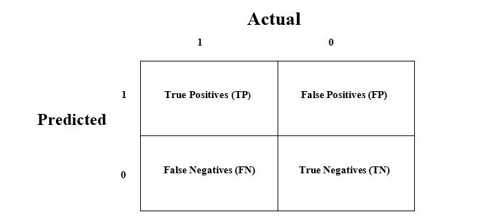
The explanation of the terms associated with confusion matrix are as follows −
- True Positives (TP) − It is the case when both actual class & predicted class of data point is 1.
- True Negatives (TN) − It is the case when both actual class & predicted class of data point is 0.
- False Positives (FP) − It is the case when actual class of data point is 0 & predicted class of data point is 1.
- False Negatives (FN) − It is the case when actual class of data point is 1 & predicted class of data point is 0.
We can find the confusion matrix with the help of confusion_matrix() function of sklearn. With the help of the following script, we can find the confusion matrix of above built binary classifier −
from sklearn.metrics import confusion_matrix
preds = gnb.predict(test)
cm = confusion_matrix(test, preds)
print(cm)
Output
[
   [ 73   7]
   [  4 144]
]
Accuracy
It may be defined as the number of correct predictions made by our ML model. We can easily calculate it by confusion matrix with the help of following formula −
$$\mathrm{Accuracy=\frac{TP+TN}{TP+FP+FN+TN}}$$
For above built binary classifier, TP + TN = 73+144 = 217 and TP+FP+FN+TN = 73+7+4+144=228.
Hence, Accuracy = 217/228 = 0.951754385965 which is same as we have calculated after creating our binary classifier.
Precision
Precision, used in document retrievals, may be defined as the number of correct documents returned by our ML model. We can easily calculate it by confusion matrix with the help of following formula −
$$\mathrm{Precision=\frac{TP}{TP+FP}}$$
For the above built binary classifier, TP = 73 and TP+FP = 73+7 = 80.
Hence, Precision = 73/80 = 0.915
Recall or Sensitivity
Recall may be defined as the number of positives returned by our ML model. We can easily calculate it by confusion matrix with the help of following formula −
$$\mathrm{Recall=\frac{TP}{TP+FN}}$$
For above built binary classifier, TP = 73 and TP+FN = 73+4 = 77.
Hence, Precision = 73/77 = 0.94805
Specificity
Specificity, in contrast to recall, may be defined as the number of negatives returned by our ML model. We can easily calculate it by confusion matrix with the help of following formula −
$$\mathrm{Specificity=\frac{TN}{TN+FP}}$$
For the above built binary classifier, TN = 144 and TN+FP = 144+7 = 151.
Hence, Precision = 144/151 = 0.95364
In the subsequent chapters, we will discuss some of the most popular classification algorithms in machine learning in detail.
