- ML - Home
- ML - Introduction
- ML - Getting Started
- ML - Basic Concepts
- ML - Ecosystem
- ML - Python Libraries
- ML - Applications
- ML - Life Cycle
- ML - Required Skills
- ML - Implementation
- ML - Challenges & Common Issues
- ML - Limitations
- ML - Reallife Examples
- ML - Data Structure
- ML - Mathematics
- ML - Artificial Intelligence
- ML - Neural Networks
- ML - Deep Learning
- ML - Getting Datasets
- ML - Categorical Data
- ML - Data Loading
- ML - Data Understanding
- ML - Data Preparation
- ML - Models
- ML - Supervised Learning
- ML - Unsupervised Learning
- ML - Semi-supervised Learning
- ML - Reinforcement Learning
- ML - Supervised vs. Unsupervised
- Machine Learning Data Visualization
- ML - Data Visualization
- ML - Histograms
- ML - Density Plots
- ML - Box and Whisker Plots
- ML - Correlation Matrix Plots
- ML - Scatter Matrix Plots
- Statistics for Machine Learning
- ML - Statistics
- ML - Mean, Median, Mode
- ML - Standard Deviation
- ML - Percentiles
- ML - Data Distribution
- ML - Skewness and Kurtosis
- ML - Bias and Variance
- ML - Hypothesis
- Regression Analysis In ML
- ML - Regression Analysis
- ML - Linear Regression
- ML - Simple Linear Regression
- ML - Multiple Linear Regression
- ML - Polynomial Regression
- Classification Algorithms In ML
- ML - Classification Algorithms
- ML - Logistic Regression
- ML - K-Nearest Neighbors (KNN)
- ML - Naïve Bayes Algorithm
- ML - Decision Tree Algorithm
- ML - Support Vector Machine
- ML - Random Forest
- ML - Confusion Matrix
- ML - Stochastic Gradient Descent
- Clustering Algorithms In ML
- ML - Clustering Algorithms
- ML - Centroid-Based Clustering
- ML - K-Means Clustering
- ML - K-Medoids Clustering
- ML - Mean-Shift Clustering
- ML - Hierarchical Clustering
- ML - Density-Based Clustering
- ML - DBSCAN Clustering
- ML - OPTICS Clustering
- ML - HDBSCAN Clustering
- ML - BIRCH Clustering
- ML - Affinity Propagation
- ML - Distribution-Based Clustering
- ML - Agglomerative Clustering
- Dimensionality Reduction In ML
- ML - Dimensionality Reduction
- ML - Feature Selection
- ML - Feature Extraction
- ML - Backward Elimination
- ML - Forward Feature Construction
- ML - High Correlation Filter
- ML - Low Variance Filter
- ML - Missing Values Ratio
- ML - Principal Component Analysis
- Reinforcement Learning
- ML - Reinforcement Learning Algorithms
- ML - Exploitation & Exploration
- ML - Q-Learning
- ML - REINFORCE Algorithm
- ML - SARSA Reinforcement Learning
- ML - Actor-critic Method
- ML - Monte Carlo Methods
- ML - Temporal Difference
- Deep Reinforcement Learning
- ML - Deep Reinforcement Learning
- ML - Deep Reinforcement Learning Algorithms
- ML - Deep Q-Networks
- ML - Deep Deterministic Policy Gradient
- ML - Trust Region Methods
- Quantum Machine Learning
- ML - Quantum Machine Learning
- ML - Quantum Machine Learning with Python
- Machine Learning Miscellaneous
- ML - Performance Metrics
- ML - Automatic Workflows
- ML - Boost Model Performance
- ML - Gradient Boosting
- ML - Bootstrap Aggregation (Bagging)
- ML - Cross Validation
- ML - AUC-ROC Curve
- ML - Grid Search
- ML - Data Scaling
- ML - Train and Test
- ML - Association Rules
- ML - Apriori Algorithm
- ML - Gaussian Discriminant Analysis
- ML - Cost Function
- ML - Bayes Theorem
- ML - Precision and Recall
- ML - Adversarial
- ML - Stacking
- ML - Epoch
- ML - Perceptron
- ML - Regularization
- ML - Overfitting
- ML - P-value
- ML - Entropy
- ML - MLOps
- ML - Data Leakage
- ML - Monetizing Machine Learning
- ML - Types of Data
- Machine Learning - Resources
- ML - Quick Guide
- ML - Cheatsheet
- ML - Interview Questions
- ML - Useful Resources
- ML - Discussion
Support Vector Machine (SVM) in Machine Learning
What is Support Vector Machine (SVM)
Support vector machines (SVMs) are powerful yet flexible supervised machine learning algorithm which is used for both classification and regression. But generally, they are used in classification problems. In 1960s, SVMs were first introduced but later they got refined in 1990 also. SVMs have their unique way of implementation as compared to other machine learning algorithms. Now a days, they are extremely popular because of their ability to handle multiple continuous and categorical variables.
Working of SVM
The goal of SVM is to find a hyperplane that separates the data points into different classes. A hyperplane is a line in 2D space, a plane in 3D space, or a higher-dimensional surface in n-dimensional space. The hyperplane is chosen in such a way that it maximizes the margin, which is the distance between the hyperplane and the closest data points of each class. The closest data points are called the support vectors.
The distance between the hyperplane and a data point "x" can be calculated using the formula −
distance = (w . x + b) / ||w||
where "w" is the weight vector, "b" is the bias term, and "||w||" is the Euclidean norm of the weight vector. The weight vector "w" is perpendicular to the hyperplane and determines its orientation, while the bias term "b" determines its position.
The optimal hyperplane is found by solving an optimization problem, which is to maximize the margin subject to the constraint that all data points are correctly classified. In other words, we want to find the hyperplane that maximizes the margin between the two classes while ensuring that no data point is misclassified. This is a convex optimization problem that can be solved using quadratic programming.
If the data points are not linearly separable, we can use a technique called kernel trick to map the data points into a higher-dimensional space where they become separable. The kernel function computes the inner product between the mapped data points without computing the mapping itself. This allows us to work with the data points in the higherdimensional space without incurring the computational cost of mapping them.
Let's understand it in detail with the help of following diagram −
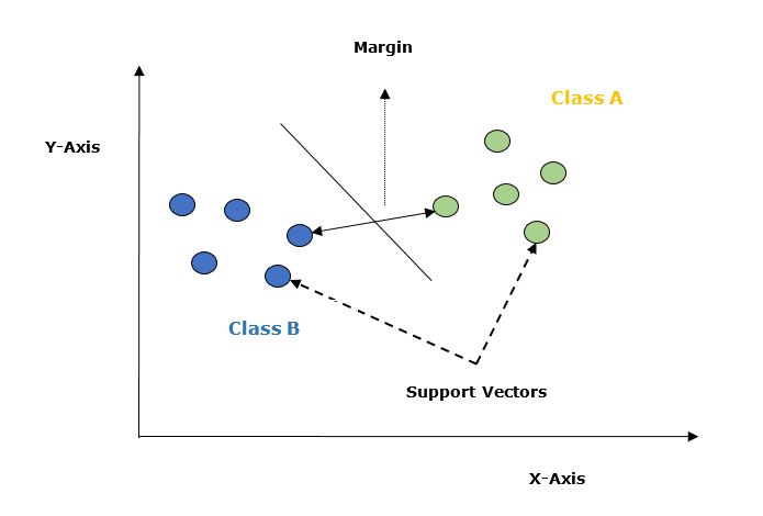
Given below are the important concepts in SVM −
Support Vectors − Datapoints that are closest to the hyperplane is called support vectors. Separating line will be defined with the help of these data points.
Hyperplane − As we can see in the above diagram it is a decision plane or space which is divided between a set of objects having different classes.
Margin − It may be defined as the gap between two lines on the closet data points of different classes. It can be calculated as the perpendicular distance from the line to the support vectors. Large margin is considered as a good margin and small margin is considered as a bad margin.
Implementing SVM Using Python
For implementing SVM in Python we will start with the standard libraries import as follows −
import numpy as np
import matplotlib.pyplot as plt
from scipy import stats
import seaborn as sns; sns.set()
Next, we are creating a sample dataset, having linearly separable data, from sklearn.dataset.sample_generator for classification using SVM −
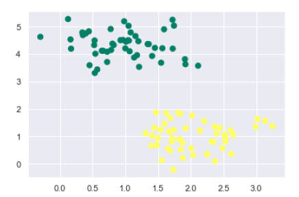
from sklearn.datasets import make_blobs
X, y = make_blobs(n_samples=100, centers=2, random_state=0, cluster_std=0.50)
plt.scatter(X[:, 0], X[:, 1], c=y, s=50, cmap='summer');
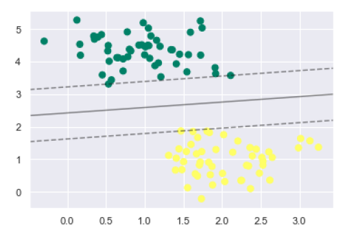
The following would be the output after generating sample dataset having 100 samples and 2 clusters −
We know that SVM supports discriminative classification. it divides the classes from each other by simply finding a line in case of two dimensions or manifold in case of multiple dimensions. It is implemented on the above dataset as follows −
xfit = np.linspace(-1, 3.5)
plt.scatter(X[:, 0], X[:, 1], c=y, s=50, cmap='summer')
plt.plot([0.6], [2.1], 'x', color='black', markeredgewidth=4, markersize=12)
for m, b in [(1, 0.65), (0.5, 1.6), (-0.2, 2.9)]:
   plt.plot(xfit, m * xfit + b, '-k')
plt.xlim(-1, 3.5);
The output is as follows −
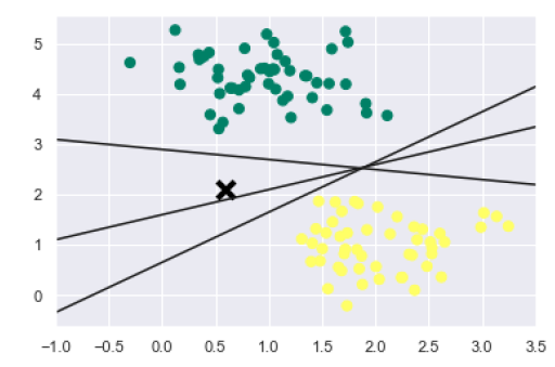
We can see from the above output that there are three different separators that perfectly discriminate the above samples.
As discussed, the main goal of SVM is to divide the datasets into classes to find a maximum marginal hyperplane (MMH) hence rather than drawing a zero line between classes we can draw around each line a margin of some width up to the nearest point. It can be done as follows −
xfit = np.linspace(-1, 3.5)
plt.scatter(X[:, 0], X[:, 1], c=y, s=50, cmap='summer')
for m, b, d in [(1, 0.65, 0.33), (0.5, 1.6, 0.55), (-0.2, 2.9, 0.2)]:
  yfit = m * xfit + b
  plt.plot(xfit, yfit, '-k')
  plt.fill_between(xfit, yfit - d, yfit + d, edgecolor='none',
        color='#AAAAAA', alpha=0.4)
  plt.xlim(-1, 3.5);
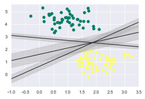
From the above image in output, we can easily observe the "margins" within the discriminative classifiers. SVM will choose the line that maximizes the margin.
Next, we will use Scikit-Learn's support vector classifier to train an SVM model on this data. Here, we are using linear kernel to fit SVM as follows −
from sklearn.svm import SVC # "Support vector classifier"
model = SVC(kernel='linear', C=1E10)
model.fit(X, y)
The output is as follows −
SVC(C=10000000000.0, cache_size=200, class_weight=None, coef0=0.0,
decision_function_shape='ovr', degree=3, gamma='auto_deprecated',
kernel='linear', max_iter=-1, probability=False, random_state=None,
shrinking=True, tol=0.001, verbose=False)
Now, for a better understanding, the following will plot the decision functions for 2D SVC −
def decision_function(model, ax=None, plot_support=True):
   if ax is None:
      ax = plt.gca()
   xlim = ax.get_xlim()
   ylim = ax.get_ylim()
For evaluating model, we need to create grid as follows −
x = np.linspace(xlim[0], xlim[1], 30)
y = np.linspace(ylim[0], ylim[1], 30)
Y, X = np.meshgrid(y, x)
xy = np.vstack([X.ravel(), Y.ravel()]).T
P = model.decision_function(xy).reshape(X.shape)
Next, we need to plot decision boundaries and margins as follows −
ax.contour(X, Y, P, colors='k',
   levels=[-1, 0, 1], alpha=0.5,
   linestyles=['--', '-', '--'])
Now, similarly plot the support vectors as follows −
if plot_support:
   ax.scatter(model.support_vectors_[:, 0],
      model.support_vectors_[:, 1],
      s=300, linewidth=1, facecolors='none');
ax.set_xlim(xlim)
ax.set_ylim(ylim)
Now, use this function to fit our models as follows −
plt.scatter(X[:, 0], X[:, 1], c=y, s=50, cmap='summer')
decision_function(model);
We can observe from the above output that an SVM classifier fit to the data with margins i.e. dashed lines and support vectors, the pivotal elements of this fit, touching the dashed line. These support vector points are stored in the support_vectors_ attribute of the classifier as follows −
model.support_vectors_
The output is as follows −
array([[0.5323772 , 3.31338909],
   [2.11114739, 3.57660449],
   [1.46870582, 1.86947425]])
SVM Kernels
In practice, SVM algorithm is implemented with kernel that transforms an input data space into the required form. SVM uses a technique called the kernel trick in which kernel takes a low dimensional input space and transforms it into a higher dimensional space. In simple words, kernel converts non-separable problems into separable problems by adding more dimensions to it. It makes SVM more powerful, flexible and accurate. The following are some of the types of kernels used by SVM −
Linear Kernel
It can be used as a dot product between any two observations. The formula of linear kernel is as below −
k(x,xi) = sum(x*xi)
From the above formula, we can see that the product between two vectors say & is the sum of the multiplication of each pair of input values.
Polynomial Kernel
It is more generalized form of linear kernel and distinguish curved or nonlinear input space. Following is the formula for polynomial kernel −
K(x, xi) = 1 + sum(x * xi)^d
Here d is the degree of polynomial, which we need to specify manually in the learning algorithm.
Radial Basis Function (RBF) Kernel
RBF kernel, mostly used in SVM classification, maps input space in indefinite dimensional space. Following formula explains it mathematically −
K(x,xi) = exp(-gamma * sum((x xi^2))
Here, gamma ranges from 0 to 1. We need to manually specify it in the learning algorithm. A good default value of gamma is 0.1.
As we implemented SVM for linearly separable data, we can implement it in Python for the data that is not linearly separable. It can be done by using kernels.
Example
The following is an example for creating an SVM classifier by using kernels. We will be using iris dataset from scikit-learn −
We will start by importing following packages −
import pandas as pd
import numpy as np
from sklearn import svm, datasets
import matplotlib.pyplot as plt
Now, we need to load the input data −
iris = datasets.load_iris()
From this dataset, we are taking first two features as follows −
X = iris.data[:, :2]
y = iris.target
Next, we will plot the SVM boundaries with original data as follows −
x_min, x_max = X[:, 0].min() - 1, X[:, 0].max() + 1
y_min, y_max = X[:, 1].min() - 1, X[:, 1].max() + 1
h = (x_max / x_min)/100
xx, yy = np.meshgrid(np.arange(x_min, x_max, h),
   np.arange(y_min, y_max, h))
X_plot = np.c_[xx.ravel(), yy.ravel()]
Now, we need to provide the value of regularization parameter as follows −
C = 1.0
Next, SVM classifier object can be created as follows −
Svc_classifier = svm.SVC(kernel='linear', C=C).fit(X, y)
Z = svc_classifier.predict(X_plot)
Z = Z.reshape(xx.shape)
plt.figure(figsize=(15, 5))
plt.subplot(121)
plt.contourf(xx, yy, Z, cmap=plt.cm.tab10, alpha=0.3)
plt.scatter(X[:, 0], X[:, 1], c=y, cmap=plt.cm.Set1)
plt.xlabel('Sepal length')
plt.ylabel('Sepal width')
plt.xlim(xx.min(), xx.max())
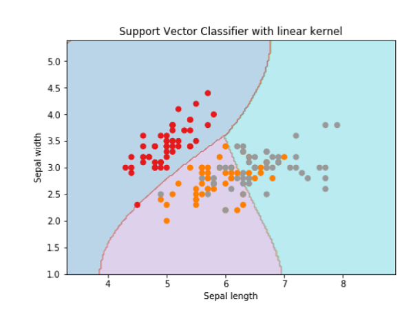
plt.title('Support Vector Classifier with linear kernel')
Output
Text(0.5, 1.0, 'Support Vector Classifier with linear kernel')
For creating SVM classifier with rbf kernel, we can change the kernel to rbf as follows −
Svc_classifier = svm.SVC(kernel='rbf', gamma ='auto',C=C).fit(X, y)
Z = svc_classifier.predict(X_plot)
Z = Z.reshape(xx.shape)
plt.figure(figsize=(15, 5))
plt.subplot(121)
plt.contourf(xx, yy, Z, cmap=plt.cm.tab10, alpha=0.3)
plt.scatter(X[:, 0], X[:, 1], c=y, cmap=plt.cm.Set1)
plt.xlabel('Sepal length')
plt.ylabel('Sepal width')
plt.xlim(xx.min(), xx.max())
plt.title('Support Vector Classifier with rbf kernel')
Output
Text(0.5, 1.0, 'Support Vector Classifier with rbf kernel')
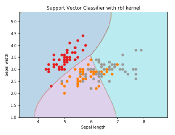
We put the value of gamma to 'auto' but you can provide its value between 0 to 1 also.
Tuning SVM Parameters
In practice, SVMs often require tuning of their parameters to achieve optimal performance. The most important parameters to tune are the kernel, the regularization parameter C, and the kernel-specific parameters.
The kernel parameter determines the type of kernel to use. The most common kernel types are linear, polynomial, radial basis function (RBF), and sigmoid. The linear kernel is used for linearly separable data, while the other kernels are used for non-linearly separable data.
The regularization parameter C controls the trade-off between maximizing the margin and minimizing the classification error. A higher value of C means that the classifier will try to minimize the classification error at the expense of a smaller margin, while a lower value of C means that the classifier will try to maximize the margin even if it means more misclassifications.
The kernel-specific parameters depend on the type of kernel being used. For example, the polynomial kernel has parameters for the degree of the polynomial and the coefficient of the polynomial, while the RBF kernel has a parameter for the width of the Gaussian function.
We can use cross-validation to tune the parameters of the SVM. Cross-validation involves splitting the data into several subsets and training the classifier on each subset while using the remaining subsets for testing. This allows us to evaluate the performance of the classifier on different subsets of the data and choose the best set of parameters.
Example
from sklearn.model_selection import GridSearchCV
# define the parameter grid
param_grid = {
   'C': [0.1, 1, 10, 100],
   'kernel': ['linear', 'poly', 'rbf', 'sigmoid'],
   'degree': [2, 3, 4],
   'coef0': [0.0, 0.1, 0.5],
   'gamma': ['scale', 'auto']
}

# create an SVM classifier
svm = SVC()

# perform grid search to find the best set of parameters
grid_search = GridSearchCV(svm, param_grid, cv=5)
grid_search.fit(X_train, y_train)
# print the best set of parameters and their accuracy
print("Best parameters:", grid_search.best_params_)
print("Best accuracy:", grid_search.best_score_)
We start by importing the GridSearchCV module from scikit-learn, which is a tool for performing grid search on a set of parameters. We define a parameter grid that contains the possible values for each parameter we want to tune.
We create an SVM classifier using SVC() and then pass it to GridSearchCV along with the parameter grid and the number of cross-validation folds (cv=5). We then call grid_search.fit(X_train, y_train) to perform the grid search.
Once the grid search is complete, we print the best set of parameters and their accuracy using grid_search.best_params_ and grid_search.best_score_, respectively.
Output
On executing this program, you will get the following output −
Best parameters: {'C': 0.1, 'coef0': 0.5, 'degree': 3, 'gamma': 'scale', 'kernel': 'poly'}
Best accuracy: 0.975
This means that the best set of parameters found by the grid search are: C=0.1, coef0=0.5, degree=3, gamma=scale, and kernel=poly. The accuracy achieved by this set of parameters on the training set is 97.5%.
You can now use these parameters to create a new SVM classifier and test its performance on the testing set.
Pros and Cons of SVM Classifiers
Pros of SVM classifiers
SVM classifiers offers great accuracy and work well with high dimensional space. SVM classifiers basically use a subset of training points hence in result uses very less memory.
Cons of SVM classifiers
They have high training time hence in practice not suitable for large datasets. Another disadvantage is that SVM classifiers do not work well with overlapping classes.
