- ML - Home
- ML - Introduction
- ML - Getting Started
- ML - Basic Concepts
- ML - Ecosystem
- ML - Python Libraries
- ML - Applications
- ML - Life Cycle
- ML - Required Skills
- ML - Implementation
- ML - Challenges & Common Issues
- ML - Limitations
- ML - Reallife Examples
- ML - Data Structure
- ML - Mathematics
- ML - Artificial Intelligence
- ML - Neural Networks
- ML - Deep Learning
- ML - Getting Datasets
- ML - Categorical Data
- ML - Data Loading
- ML - Data Understanding
- ML - Data Preparation
- ML - Models
- ML - Supervised Learning
- ML - Unsupervised Learning
- ML - Semi-supervised Learning
- ML - Reinforcement Learning
- ML - Supervised vs. Unsupervised
- Machine Learning Data Visualization
- ML - Data Visualization
- ML - Histograms
- ML - Density Plots
- ML - Box and Whisker Plots
- ML - Correlation Matrix Plots
- ML - Scatter Matrix Plots
- Statistics for Machine Learning
- ML - Statistics
- ML - Mean, Median, Mode
- ML - Standard Deviation
- ML - Percentiles
- ML - Data Distribution
- ML - Skewness and Kurtosis
- ML - Bias and Variance
- ML - Hypothesis
- Regression Analysis In ML
- ML - Regression Analysis
- ML - Linear Regression
- ML - Simple Linear Regression
- ML - Multiple Linear Regression
- ML - Polynomial Regression
- Classification Algorithms In ML
- ML - Classification Algorithms
- ML - Logistic Regression
- ML - K-Nearest Neighbors (KNN)
- ML - Naïve Bayes Algorithm
- ML - Decision Tree Algorithm
- ML - Support Vector Machine
- ML - Random Forest
- ML - Confusion Matrix
- ML - Stochastic Gradient Descent
- Clustering Algorithms In ML
- ML - Clustering Algorithms
- ML - Centroid-Based Clustering
- ML - K-Means Clustering
- ML - K-Medoids Clustering
- ML - Mean-Shift Clustering
- ML - Hierarchical Clustering
- ML - Density-Based Clustering
- ML - DBSCAN Clustering
- ML - OPTICS Clustering
- ML - HDBSCAN Clustering
- ML - BIRCH Clustering
- ML - Affinity Propagation
- ML - Distribution-Based Clustering
- ML - Agglomerative Clustering
- Dimensionality Reduction In ML
- ML - Dimensionality Reduction
- ML - Feature Selection
- ML - Feature Extraction
- ML - Backward Elimination
- ML - Forward Feature Construction
- ML - High Correlation Filter
- ML - Low Variance Filter
- ML - Missing Values Ratio
- ML - Principal Component Analysis
- Reinforcement Learning
- ML - Reinforcement Learning Algorithms
- ML - Exploitation & Exploration
- ML - Q-Learning
- ML - REINFORCE Algorithm
- ML - SARSA Reinforcement Learning
- ML - Actor-critic Method
- ML - Monte Carlo Methods
- ML - Temporal Difference
- Deep Reinforcement Learning
- ML - Deep Reinforcement Learning
- ML - Deep Reinforcement Learning Algorithms
- ML - Deep Q-Networks
- ML - Deep Deterministic Policy Gradient
- ML - Trust Region Methods
- Quantum Machine Learning
- ML - Quantum Machine Learning
- ML - Quantum Machine Learning with Python
- Machine Learning Miscellaneous
- ML - Performance Metrics
- ML - Automatic Workflows
- ML - Boost Model Performance
- ML - Gradient Boosting
- ML - Bootstrap Aggregation (Bagging)
- ML - Cross Validation
- ML - AUC-ROC Curve
- ML - Grid Search
- ML - Data Scaling
- ML - Train and Test
- ML - Association Rules
- ML - Apriori Algorithm
- ML - Gaussian Discriminant Analysis
- ML - Cost Function
- ML - Bayes Theorem
- ML - Precision and Recall
- ML - Adversarial
- ML - Stacking
- ML - Epoch
- ML - Perceptron
- ML - Regularization
- ML - Overfitting
- ML - P-value
- ML - Entropy
- ML - MLOps
- ML - Data Leakage
- ML - Monetizing Machine Learning
- ML - Types of Data
- Machine Learning - Resources
- ML - Quick Guide
- ML - Cheatsheet
- ML - Interview Questions
- ML - Useful Resources
- ML - Discussion
Machine Learning - Hierarchical Clustering
Hierarchical Clustering
Hierarchical clustering is an unsupervised learning algorithm that is used to group together the unlabeled data points having similar characteristics. Hierarchical clustering algorithms falls into following two categories −
- Agglomerative hierarchical algorithms − In agglomerative hierarchical algorithms, each data point is treated as a single cluster and then successively merge or agglomerate (bottom-up approach) the pairs of clusters. The hierarchy of the clusters is represented as a dendrogram or tree structure.
- Divisive hierarchical algorithms − On the other hand, in divisive hierarchical algorithms, all the data points are treated as one big cluster and the process of clustering involves dividing (Top-down approach) the one big cluster into various small clusters.
Steps to Perform Agglomerative Hierarchical Clustering
We are going to explain the most used and important Hierarchical clustering i.e. agglomerative. The steps to perform the same is as follows −
- Step 1 − Treat each data point as single cluster. Hence, we will be having say K clusters at start. The number of data points will also be K at start.
- Step 2 − Now, in this step we need to form a big cluster by joining two closet datapoints. This will result in total of K-1 clusters.
- Step 3 − Now, to form more clusters we need to join two closet clusters. This will result in total of K-2 clusters.
- Step 4 − Now, to form one big cluster repeat the above three steps until K would become 0 i.e. no more data points left to join.
- Step 5 − At last, after making one single big cluster, dendrograms will be used to divide into multiple clusters depending upon the problem.
Role of Dendrograms in Agglomerative Hierarchical Clustering
As we discussed in the last step, the role of dendrogram started once the big cluster is formed. Dendrogram will be used to split the clusters into multiple cluster of related data points depending upon our problem. It can be understood with the help of following example −
Example - Dendrograms
To understand, let's start with importing the required libraries as follows −
%matplotlib inline
import matplotlib.pyplot as plt
import numpy as np
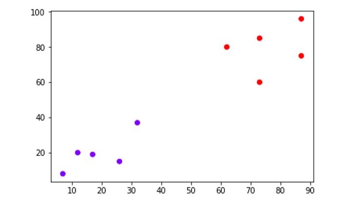
Next, we will be plotting the datapoints we have taken for this example −
%matplotlib inline
import matplotlib.pyplot as plt
import numpy as np

X = np.array([[7,8],[12,20],[17,19],[26,15],[32,37],[87,75],[73,85],
[62,80],[73,60],[87,96],])
labels = range(1, 11)
plt.figure(figsize=(10, 7))
plt.subplots_adjust(bottom=0.1)
plt.scatter(X[:,0],X[:,1], label='True Position')

for label, x, y in zip(labels, X[:, 0], X[:, 1]):
   plt.annotate(label,xy=(x, y), xytext=(-3, 3),textcoords='offset points', ha='right', va='bottom')
plt.show()
Output
When you execute this code, it will produce the following plot as the output −
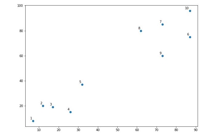
From the above diagram, it is very easy to see we have two clusters in our datapoints but in real-world data, there can be thousands of clusters.
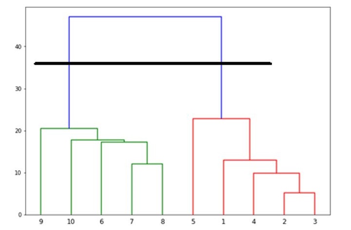
Next, we will be plotting the dendrograms of our datapoints by using Scipy library −
from scipy.cluster.hierarchy import dendrogram, linkage
from matplotlib import pyplot as plt
linked = linkage(X, 'single')
labelList = range(1, 11)
plt.figure(figsize=(10, 7))

dendrogram(linked, orientation='top',labels=labelList,
distance_sort='descending',show_leaf_counts=True)

plt.show()
Output
It will produce the following plot −
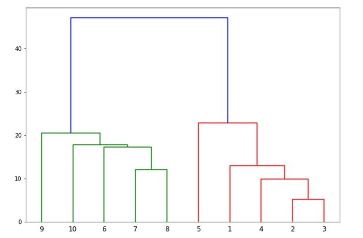
Now, once the big cluster is formed, the longest vertical distance is selected. A vertical line is then drawn through it as shown in the following diagram. As the horizontal line crosses the blue line at two points hence the number of clusters would be two.
Next, we need to import the class for clustering and call its fit_predict method to predict the cluster. We are importing AgglomerativeClustering class of sklearn.cluster library −
from sklearn.cluster import AgglomerativeClustering

cluster = AgglomerativeClustering(n_clusters=2,
linkage='ward')

cluster.fit_predict(X)
Next, plot the cluster with the help of following code −
from sklearn.cluster import AgglomerativeClustering

cluster = AgglomerativeClustering(n_clusters=2,
linkage='ward')

cluster.fit_predict(X)

plt.scatter(X[:,0],X[:,1], c=cluster.labels_, cmap='rainbow')
The following diagram shows the two clusters from our datapoints.
Example - Clusters of Data Points
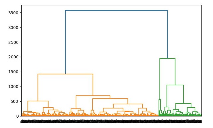
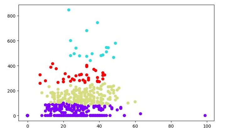
As we understood the concept of dendrograms from the simple example above, let's move to another example in which we are creating clusters of the data point in Pima Indian Diabetes Dataset by using hierarchical clustering −
import matplotlib.pyplot as plt
import pandas as pd
import numpy as np

from pandas import read_csv
path = r"C:\pima-indians-diabetes.csv"
headernames = ['preg', 'plas', 'pres', 'skin', 'test', 'mass', 'pedi', 'age', 'class']
data = read_csv(path, names=headernames)
array = data.values
X = array[:,0:8]
Y = array[:,8]

patient_data = data.iloc[:, 3:5].values
import scipy.cluster.hierarchy as shc
plt.figure(figsize=(10, 7))
plt.title("Patient Dendograms")

dend = shc.dendrogram(shc.linkage(data, method='ward'))

from sklearn.cluster import AgglomerativeClustering
cluster = AgglomerativeClustering(n_clusters=4, linkage='ward')
cluster.fit_predict(patient_data)

plt.figure(figsize=(7.2, 5.5))
plt.scatter(patient_data[:,0], patient_data[:,1], c=cluster.labels_,
cmap='rainbow')
Output
When you run this code, it will produce the following two plots as the output −