- ML - Home
- ML - Introduction
- ML - Getting Started
- ML - Basic Concepts
- ML - Ecosystem
- ML - Python Libraries
- ML - Applications
- ML - Life Cycle
- ML - Required Skills
- ML - Implementation
- ML - Challenges & Common Issues
- ML - Limitations
- ML - Reallife Examples
- ML - Data Structure
- ML - Mathematics
- ML - Artificial Intelligence
- ML - Neural Networks
- ML - Deep Learning
- ML - Getting Datasets
- ML - Categorical Data
- ML - Data Loading
- ML - Data Understanding
- ML - Data Preparation
- ML - Models
- ML - Supervised Learning
- ML - Unsupervised Learning
- ML - Semi-supervised Learning
- ML - Reinforcement Learning
- ML - Supervised vs. Unsupervised
- Machine Learning Data Visualization
- ML - Data Visualization
- ML - Histograms
- ML - Density Plots
- ML - Box and Whisker Plots
- ML - Correlation Matrix Plots
- ML - Scatter Matrix Plots
- Statistics for Machine Learning
- ML - Statistics
- ML - Mean, Median, Mode
- ML - Standard Deviation
- ML - Percentiles
- ML - Data Distribution
- ML - Skewness and Kurtosis
- ML - Bias and Variance
- ML - Hypothesis
- Regression Analysis In ML
- ML - Regression Analysis
- ML - Linear Regression
- ML - Simple Linear Regression
- ML - Multiple Linear Regression
- ML - Polynomial Regression
- Classification Algorithms In ML
- ML - Classification Algorithms
- ML - Logistic Regression
- ML - K-Nearest Neighbors (KNN)
- ML - Naïve Bayes Algorithm
- ML - Decision Tree Algorithm
- ML - Support Vector Machine
- ML - Random Forest
- ML - Confusion Matrix
- ML - Stochastic Gradient Descent
- Clustering Algorithms In ML
- ML - Clustering Algorithms
- ML - Centroid-Based Clustering
- ML - K-Means Clustering
- ML - K-Medoids Clustering
- ML - Mean-Shift Clustering
- ML - Hierarchical Clustering
- ML - Density-Based Clustering
- ML - DBSCAN Clustering
- ML - OPTICS Clustering
- ML - HDBSCAN Clustering
- ML - BIRCH Clustering
- ML - Affinity Propagation
- ML - Distribution-Based Clustering
- ML - Agglomerative Clustering
- Dimensionality Reduction In ML
- ML - Dimensionality Reduction
- ML - Feature Selection
- ML - Feature Extraction
- ML - Backward Elimination
- ML - Forward Feature Construction
- ML - High Correlation Filter
- ML - Low Variance Filter
- ML - Missing Values Ratio
- ML - Principal Component Analysis
- Reinforcement Learning
- ML - Reinforcement Learning Algorithms
- ML - Exploitation & Exploration
- ML - Q-Learning
- ML - REINFORCE Algorithm
- ML - SARSA Reinforcement Learning
- ML - Actor-critic Method
- ML - Monte Carlo Methods
- ML - Temporal Difference
- Deep Reinforcement Learning
- ML - Deep Reinforcement Learning
- ML - Deep Reinforcement Learning Algorithms
- ML - Deep Q-Networks
- ML - Deep Deterministic Policy Gradient
- ML - Trust Region Methods
- Quantum Machine Learning
- ML - Quantum Machine Learning
- ML - Quantum Machine Learning with Python
- Machine Learning Miscellaneous
- ML - Performance Metrics
- ML - Automatic Workflows
- ML - Boost Model Performance
- ML - Gradient Boosting
- ML - Bootstrap Aggregation (Bagging)
- ML - Cross Validation
- ML - AUC-ROC Curve
- ML - Grid Search
- ML - Data Scaling
- ML - Train and Test
- ML - Association Rules
- ML - Apriori Algorithm
- ML - Gaussian Discriminant Analysis
- ML - Cost Function
- ML - Bayes Theorem
- ML - Precision and Recall
- ML - Adversarial
- ML - Stacking
- ML - Epoch
- ML - Perceptron
- ML - Regularization
- ML - Overfitting
- ML - P-value
- ML - Entropy
- ML - MLOps
- ML - Data Leakage
- ML - Monetizing Machine Learning
- ML - Types of Data
- Machine Learning - Resources
- ML - Quick Guide
- ML - Cheatsheet
- ML - Interview Questions
- ML - Useful Resources
- ML - Discussion
Linear Regression in Machine Learning
Linear regression in machine learning is defined as a statistical model that analyzes the linear relationship between a dependent variable and a given set of independent variables. The linear relationship between variables means that when the value of one or more independent variables will change (increase or decrease), the value of the dependent variable will also change accordingly (increase or decrease).
In machine learning, linear regression is used for predicting continuous numeric values based on learned linear relation for new and unseen data. It is used in predictive modeling, financial forecasting, risk assessment, etc.
In this chapter, we will discuss the following topics in detail −
- What is Linear Regression?
- Types of Linear Regression
- How Does Linear Regression Work?
- Hypothesis Function For Linear Regression
- Finding the Best Fit Line
- Loss Function For Linear Regression
- Gradient Descent for Optimization
- Assumptions of Linear Regression
- Evaluation Metrics for Linear Regression
- Applications of Linear Regression
- Advantages of Linear Regression
- Common Challenges with Linear Regression
What is Linear Regression?
Linear regression is a statistical technique that estimates the linear relationship between a dependent and one or more independent variables. In machine learning, linear regression is implemented as a supervised learning approach. In machine learning, labeled datasets contain input data (features) and output labels (target values). For linear regression in machine learning, we represent features as independent variables and target values as the dependent variable.
For the simplicity, take the following data (Single feature and single target)
| Square Feet (X) | House Price (Y) |
|---|---|
| 1300 | 240 |
| 1500 | 320 |
| 1700 | 330 |
| 1830 | 295 |
| 1550 | 256 |
| 2350 | 409 |
| 1450 | 319 |
In the above data, the target House Price is the dependent variable represented by X, and the feature, Square Feet, is the independent variable represented by Y. The input features (X) are used to predict the target label (Y). So, the independent variables are also known as predictor variables, and the dependent variable is known as the response variable.
So lets define linear regression in machine learning as follows:
In machine learning, linear regression uses a linear equation to model the relationship between a dependent variable (Y) and one or more independent variables (Y).
The main goal of the linear regression model is to find the best-fitting straight line (often called a regression line) through a set of data points.
Line of Regression
A straight line that shows a relation between the dependent variable and independent variables is known as the line of regression or regression line.

Furthermore, the linear relationship can be positive or negative in nature as explained below −
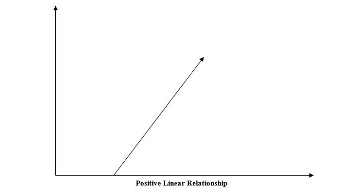
1. Positive Linear Relationship
A linear relationship will be called positive if both independent and dependent variable increases. It can be understood with the help of the following graph −
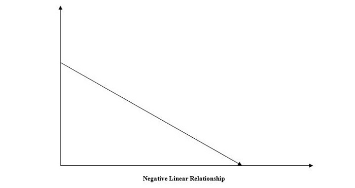
2. Negative Linear Relationship
A linear relationship will be called positive if the independent increases and the dependent variable decreases. It can be understood with the help of the following graph −
Linear regression is of two types, "simple linear regression" and "multiple linear regression", which we are going to discuss in the next two chapters of this tutorial.
Types of Linear Regression
Linear regression is of the following two types −
- Simple Linear Regression
- Multiple Linear Regression
1. Simple Linear Regression
Simple linear regression is a type of regression analysis in which a single independent variable (also known as a predictor variable) is used to predict the dependent variable. In other words, it models the linear relationship between the dependent variable and a single independent variable.

In the above image, the straight line represents the simple linear regression line where Ŷ is the predicted value, and X is the input value.
Mathematically, the relationship can be modeled as a linear equation −
$$\mathrm{ Y = w_0 + w_1 X + \epsilon }$$
Where
- Y is the dependent variable (target).
- X is the independent variable (feature).
- w0 is the y-intercept of the line.
- w1 is the slope of the line, representing the effect of X on Y.
- ε is the error term, capturing the variability in Y not explained by X.
2. Multiple Linear Regression
Multiple linear regression is basically the extension of simple linear regression that predicts a response using two or more features.
When dealing with more than one independent variable, we extend simple linear regression to multiple linear regression. The model is expressed as:
Multiple linear regression extends the concept of simple linear regression to multiple independent variables. The model is expressed as:
$$\mathrm{Y = w_0 + w_1 X_1 + w_2 X_2 + \dots + w_p X_p + \epsilon}$$
Where
- X1, X2, ..., Xp are the independent variables (features).
- w0, w1, ..., wp are the coefficients for these variables.
- ε is the error term.
How Does Linear Regression Work?
The main goal of linear regression is to find the best-fit line through a set of data points that minimizes the difference between the actual values and predicted values. So it is done? This is done by estimating the parameters w0, w1 etc.
The working of linear regression in machine learning can be broken down into many steps as follows −
- Hypothesis − We assume that there is a linear relation between input and output.
- Cost Function − Define a loss or cost function. The cost function quantifies the model's prediction error. The cost function takes the model's predicted values and actual values and returns a single scaler value that represents the cost of the model's prediction.
- Optimization − Optimize (minimize) the model's cost function by updating the model's parameters.
It continues updating the model's parameters until the cost or error of the model's prediction is optimized (minimized).
Let's discuss the above three steps in more detail −
Hypothesis Function For Linear Regression
In linear regression problems, we assume that there is a linear relationship between input features (X) and predicted value (Ŷ).
The hypothesis function returns the predicted value for a given input value. Generally we represent a hypothesis by hw(X) and it is equal to Ŷ.
Hypothesis function for simple linear regression −
$$\mathrm{\hat{Y} = w_0 + w_1 X}$$
Hypothesis function for multiple linear regression −
$$\mathrm{\hat{Y} = w_0 + w_1 X_1 + w_2 X_2 + \dots + w_p X_p}$$
For different values of parameters (weights), we can find many regression lines. The main goal is to find the best-fit lines. Let's discuss it as below −
Finding the Best Fit Line
We discussed above that different set of parameters will provide different regression lines. However, each regression line does not represent the optimal relation between the input and output values. The main goal is to find the best-fit line.
A regression line is said to be the best fit if the error between actual and predicted values is minimal.
Below image shows a regression line with error (ε) at input data point X. The error is calculated for all data points and our goal is to minimize the average error/ loss. We can use different types of loss functions such as mean square error (MSE), mean average error (MAE), L1 loss, L2 Loss, etc.

So, how can we minimize the error between the actual and predicted values? Let's discuss the important concept, which is cost function or loss function.
Loss Function for Linear Regression
The error between actual and predicted values can be quantified using a loss function of the cost function. The cost function takes the model's predicted values and actual values and returns a single scaler value that represents the cost of the model's prediction. Our main goal is to minimize the cost function.
The most commonly used cost function is the mean squared error function.
$$\mathrm{J(w_0, w_1) = \frac{1}{2n} \sum_{i=1}^{n} \left( Y_i - \hat{Y}_i \right)^2}$$
Where,
- n is the number of data points.
- Yi is the observed value for the i-th data point.
- \( \hat{Y}_i = w_0 + w_1 X_i \) is the predicted value for the i-th data point.
Gradient Descent for Optimization
Now we have defined our loss function. The next step is to minimize it and find the optimized values of the parameters or weights. This process of finding optimal values of parameters such that the loss or error is minimal is known as model optimization.
Gradient Descent is one of the most used optimization techniques for linear regression.
To find the optimal values of parameters, gradient descent is often used, especially in cases with large datasets. Gradient descent iteratively adjusts the parameters in the direction of the steepest descent of the cost function.
The parameter updates are given by
$$\mathrm{w_0 = w_0 - \alpha \frac{\partial J}{\partial w_0}}$$
$$\mathrm{w_1 = w_1 - \alpha \frac{\partial J}{\partial w_1}}$$
Where α is the learning rate, and the partial derivatives are:
$$\mathrm{\frac{\partial J}{\partial w_0} = -\frac{1}{n} \sum_{i=1}^{n} \left( Y_i - \hat{Y}_i \right)}$$
$$\mathrm{\frac{\partial J}{\partial w_1} = -\frac{1}{n} \sum_{i=1}^{n} \left( Y_i - \hat{Y}_i \right) X_i}$$
These gradients are used to update the parameters until convergence is reached (i.e., when the changes in \( w_0 \) and \( w_1 \) become negligible).
Assumptions of Linear Regression
The following are some assumptions about the dataset that are made by the Linear Regression model −
Multi-collinearity − Linear regression model assumes that there is very little or no multi-collinearity in the data. Basically, multi-collinearity occurs when the independent variables or features have a dependency on them.
Auto-correlation − Another assumption the Linear regression model assumes is that there is very little or no auto-correlation in the data. Basically, auto-correlation occurs when there is dependency between residual errors.
Relationship between variables − Linear regression model assumes that the relationship between response and feature variables must be linear.
Violations of these assumptions can lead to biased or inefficient estimates. It is essential to validate these assumptions to ensure model accuracy.
Evaluation Metrics for Linear Regression
To assess the performance of a linear regression model, several evaluation metrics are used −
R-squared (R2) − It measures the proportion of the variance in the dependent variable that is predictable from the independent variables.
$$\mathrm{ R^2 = 1 - \frac{\sum (y_i - \hat{y}_i)^2}{\sum (y_i - \bar{y})^2} }$$
Mean Squared Error (MSE) − It measures an average of the sum of the squared difference between the predicted values and the actual values.
$$\mathrm{ \text{MSE} = \frac{1}{n} \sum_{i=1}^n (y_i - \hat{y}_i)^2 }$$
Root Mean Squared Error (RMSE) − It measures the square root of the MSE.
$$\mathrm{ \text{RMSE} = \sqrt{\text{MSE}} }$$
Mean Absolute Error (MAE) − It measures the average of the sum of the absolute values of the difference between the predicted values and the actual values.
$$\mathrm{ \text{MAE} = \frac{1}{n} \sum_{i=1}^n |y_i - \hat{y}_i| }$$
Applications of Linear Regression
1. Predictive Modeling
Linear regression is widely used for predictive modeling. For instance, in real estate, predicting house prices based on features such as size, location, and number of bedrooms can help buyers, sellers, and real estate agents make informed decisions.
2. Feature Selection
In multiple linear regression, analyzing the coefficients can help in feature selection. Features with small or zero coefficients might be considered less important and can be dropped to simplify the model.
3. Financial Forecasting
In finance, linear regression models predict stock prices, economic indicators, and market trends. Accurate forecasts can guide investment strategies and financial planning.
4. Risk Management
Linear regression helps in risk assessment by modeling the relationship between risk factors and financial metrics. For example, in insurance, it can model the relationship between policyholder characteristics and claim amounts.
Advantages of Linear Regression
- Interpretability − Linear regression is easy to understand, which is useful when explaining how a model makes decisions.
- Speed − Linear regression is faster to train than many other machine learning algorithms.
- Predictive analytics − Linear regression is a fundamental building block for predictive analytics.
- Linear relationships − Linear regression is a powerful statistical method for finding linear relationships between variables.
- Simplicity − Linear regression is simple to implement and interpret.
- Efficiency − Linear regression is efficient to compute.
Common Challenges with Linear Regression
1. Overfitting
Overfitting occurs when the regression model performs well on training data but lacks generalization on test data. Overfitting leads to poor prediction on new, unseen data.
2. Multicollinearity
When the dependent variables (predictor or feature variables) correlate, the situation is known as mutilcolinearty. In this, the estimates of the parameters (coefficients) can be unstable.
3. Outliers and Their Impact
Outliers can cause the regression line to be a poor fit for the majority of data points.
Polynomial Regression: An Alternate to Linear Regression
Polynomial Linear Regression is a type of regression analysis in which the relationship between the independent variable and the dependent variable is modeled as an n-th degree polynomial function. Polynomial regression allows for a more complex relationship between the variables to be captured beyond the linear relationship in Simple and Multiple Linear Regression.
