ML - Implementing SVM in Python

For implementing SVM in Python we will start with the standard libraries import as follows −

import numpy as np
import matplotlib.pyplot as plt
from scipy import stats
import seaborn as sns; sns.set()

Next, we are creating a sample dataset, having linearly separable data, from sklearn.dataset.sample_generator for classification using SVM −

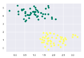
from sklearn.datasets.samples_generator import make_blobs
X, y = make_blobs(n_samples = 100, centers = 2, random_state = 0, cluster_std = 0.50)
plt.scatter(X[:, 0], X[:, 1], c = y, s = 50, cmap = 'summer');

The following would be the output after generating sample dataset having 100 samples and 2 clusters −

We know that SVM supports discriminative classification. it divides the classes from each other by simply finding a line in case of two dimensions or manifold in case of multiple dimensions. It is implemented on the above dataset as follows −

xfit = np.linspace(-1, 3.5)
plt.scatter(X[:, 0], X[:, 1], c = y, s = 50, cmap = 'summer')
plt.plot([0.6], [2.1], 'x', color = 'black', markeredgewidth = 4, markersize = 12)
for m, b in [(1, 0.65), (0.5, 1.6), (-0.2, 2.9)]:
plt.plot(xfit, m * xfit + b, '-k')
plt.xlim(-1, 3.5);

The output is as follows −

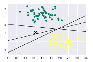
We can see from the above output that there are three different separators that perfectly discriminate the above samples.

As discussed, the main goal of SVM is to divide the datasets into classes to find a maximum marginal hyperplane (MMH) hence rather than drawing a zero line between classes we can draw around each line a margin of some width up to the nearest point. It can be done as follows −

xfit = np.linspace(-1, 3.5)
plt.scatter(X[:, 0], X[:, 1], c = y, s = 50, cmap = 'summer')

for m, b, d in [(1, 0.65, 0.33), (0.5, 1.6, 0.55), (-0.2, 2.9, 0.2)]:
   yfit = m * xfit + b
   plt.plot(xfit, yfit, '-k')
   plt.fill_between(xfit, yfit - d, yfit + d, edgecolor='none',
   color = '#AAAAAA', alpha = 0.4)
plt.xlim(-1, 3.5);

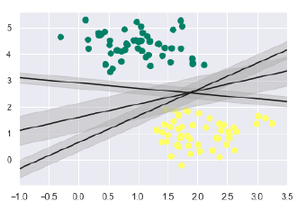
From the above image in output, we can easily observe the “margins” within the discriminative classifiers. SVM will choose the line that maximizes the margin.

Next, we will use Scikit-Learn’s support vector classifier to train an SVM model on this data. Here, we are using linear kernel to fit SVM as follows −

from sklearn.svm import SVC # "Support vector classifier"
model = SVC(kernel = 'linear', C = 1E10)
model.fit(X, y)

The output is as follows −

SVC(C=10000000000.0, cache_size=200, class_weight=None, coef0=0.0,
decision_function_shape='ovr', degree=3, gamma='auto_deprecated',
kernel='linear', max_iter=-1, probability=False, random_state=None,
shrinking=True, tol=0.001, verbose=False)

Now, for a better understanding, the following will plot the decision functions for 2D SVC −

def decision_function(model, ax = None, plot_support = True):
   if ax is None:
      ax = plt.gca()
   xlim = ax.get_xlim()
   ylim = ax.get_ylim()

For evaluating model, we need to create grid as follows −

x = np.linspace(xlim[0], xlim[1], 30)
y = np.linspace(ylim[0], ylim[1], 30)
Y, X = np.meshgrid(y, x)
xy = np.vstack([X.ravel(), Y.ravel()]).T
P = model.decision_function(xy).reshape(X.shape)

Next, we need to plot decision boundaries and margins as follows −

ax.contour(X, Y, P, colors = 'k', levels = [-1, 0, 1], alpha = 0.5, linestyles = ['--', '-', '--'])

Now, similarly plot the support vectors as follows −

if plot_support:
   ax.scatter(model.support_vectors_[:, 0],
   model.support_vectors_[:, 1], s = 300, linewidth = 1, facecolors = 'none');
ax.set_xlim(xlim)
ax.set_ylim(ylim)

Now, use this function to fit our models as follows −

plt.scatter(X[:, 0], X[:, 1], c = y, s = 50, cmap = 'summer')
decision_function(model);

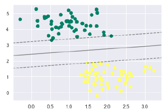
We can observe from the above output that an SVM classifier fit to the data with margins i.e. dashed lines and support vectors, the pivotal elements of this fit, touching the dashed line. These support vector points are stored in the support_vectors_ attribute of the classifier as follows −

model.support_vectors_

The output is as follows −

array([[0.5323772 , 3.31338909], [2.11114739, 3.57660449], [1.46870582, 1.86947425]])