- Home
- Basics
- Python Ecosystem
- Methods for Machine Learning
- Data Loading for ML Projects
- Understanding Data with Statistics
- Understanding Data with Visualization
- Preparing Data
- Data Feature Selection
- ML Algorithms - Classification
- Introduction
- Logistic Regression
- Support Vector Machine (SVM)
- Decision Tree
- Naïve Bayes
- Random Forest
- ML Algorithms - Regression
- Random Forest
- Linear Regression
- ML Algorithms - Clustering
- Overview
- K-means Algorithm
- Mean Shift Algorithm
- Hierarchical Clustering
- ML Algorithms - KNN Algorithm
- Finding Nearest Neighbors
- Performance Metrics
- Automatic Workflows
- Improving Performance of ML Models
- Improving Performance of ML Model (Contd…)
- ML With Python - Resources
- Machine Learning With Python - Quick Guide
- Machine Learning with Python - Resources
- Machine Learning With Python - Discussion
Data Preprocessing, Analysis & Visualization
In the real world, we usually come across lots of raw data which is not fit to be readily processed by machine learning algorithms. We need to preprocess the raw data before it is fed into various machine learning algorithms. This chapter discusses various techniques for preprocessing data in Python machine learning.
Data Preprocessing
In this section, let us understand how we preprocess data in Python.
Initially, open a file with a .py extension, for example prefoo.py file, in a text editor like notepad.
Then, add the following piece of code to this file −
import numpy as np

from sklearn import preprocessing

#We imported a couple of packages. Let's create some sample data and add the line to this file:

input_data = np.array([[3, -1.5, 3, -6.4], [0, 3, -1.3, 4.1], [1, 2.3, -2.9, -4.3]])
We are now ready to operate on this data.
Preprocessing Techniques
Data can be preprocessed using several techniques as discussed here −
Mean removal
It involves removing the mean from each feature so that it is centered on zero. Mean removal helps in removing any bias from the features.
You can use the following code for mean removal −
data_standardized = preprocessing.scale(input_data)
print "\nMean = ", data_standardized.mean(axis = 0)
print "Std deviation = ", data_standardized.std(axis = 0)
Now run the following command on the terminal −
$ python prefoo.py
You can observe the following output −
Mean = [ 5.55111512e-17 -3.70074342e-17 0.00000000e+00 -1.85037171e-17]
Std deviation = [1. 1. 1. 1.]
Observe that in the output, mean is almost 0 and the standard deviation is 1.
Scaling
The values of every feature in a data point can vary between random values. So, it is important to scale them so that this matches specified rules.
You can use the following code for scaling −
data_scaler = preprocessing.MinMaxScaler(feature_range = (0, 1))
data_scaled = data_scaler.fit_transform(input_data)
print "\nMin max scaled data = ", data_scaled
Now run the code and you can observe the following output −
Min max scaled data = [ [ 1. 0. 1. 0. ]
                        [ 0. 1. 0.27118644 1. ]
                        [ 0.33333333 0.84444444 0. 0.2 ]
]
Note that all the values have been scaled between the given range.
Normalization
Normalization involves adjusting the values in the feature vector so as to measure them on a common scale. Here, the values of a feature vector are adjusted so that they sum up to 1. We add the following lines to the prefoo.py file −
You can use the following code for normalization −
data_normalized = preprocessing.normalize(input_data, norm  = 'l1')
print "\nL1 normalized data = ", data_normalized
Now run the code and you can observe the following output −
L1 normalized data = [  [ 0.21582734 -0.10791367 0.21582734 -0.46043165]
                        [ 0. 0.35714286 -0.1547619 0.48809524]
                        [ 0.0952381 0.21904762 -0.27619048 -0.40952381]
]
Normalization is used to ensure that data points do not get boosted due to the nature of their features.
Binarization
Binarization is used to convert a numerical feature vector into a Boolean vector. You can use the following code for binarization −
data_binarized = preprocessing.Binarizer(threshold=1.4).transform(input_data)
print "\nBinarized data =", data_binarized
Now run the code and you can observe the following output −
Binarized data = [[ 1. 0. 1. 0.]
                  [ 0. 1. 0. 1.]
                  [ 0. 1. 0. 0.]
                 ]
This technique is helpful when we have prior knowledge of the data.
One Hot Encoding
It may be required to deal with numerical values that are few and scattered, and you may not need to store these values. In such situations you can use One Hot Encoding technique.
If the number of distinct values is k, it will transform the feature into a k-dimensional vector where only one value is 1 and all other values are 0.
You can use the following code for one hot encoding −
encoder = preprocessing.OneHotEncoder()
encoder.fit([  [0, 2, 1, 12],
               [1, 3, 5, 3],
               [2, 3, 2, 12],
               [1, 2, 4, 3]
])
encoded_vector = encoder.transform([[2, 3, 5, 3]]).toarray()
print "\nEncoded vector =", encoded_vector
Now run the code and you can observe the following output −
Encoded vector = [[ 0. 0. 1. 0. 1. 0. 0. 0. 1. 1. 0.]]
In the example above, let us consider the third feature in each feature vector. The values are 1, 5, 2, and 4.
There are four separate values here, which means the one-hot encoded vector will be of length 4. If we want to encode the value 5, it will be a vector [0, 1, 0, 0]. Only one value can be 1 in this vector. The second element is 1, which indicates that the value is 5.
Label Encoding
In supervised learning, we mostly come across a variety of labels which can be in the form of numbers or words. If they are numbers, then they can be used directly by the algorithm. However, many times, labels need to be in readable form. Hence, the training data is usually labelled with words.
Label encoding refers to changing the word labels into numbers so that the algorithms can understand how to work on them. Let us understand in detail how to perform label encoding −
Create a new Python file, and import the preprocessing package −
from sklearn import preprocessing
label_encoder = preprocessing.LabelEncoder()
input_classes = ['suzuki', 'ford', 'suzuki', 'toyota', 'ford', 'bmw']
label_encoder.fit(input_classes)
print "\nClass mapping:"
for i, item in enumerate(label_encoder.classes_):
print item, '-->', i
Now run the code and you can observe the following output −
Class mapping:
bmw --> 0
ford --> 1
suzuki --> 2
toyota --> 3
As shown in above output, the words have been changed into 0-indexed numbers. Now, when we deal with a set of labels, we can transform them as follows −
labels = ['toyota', 'ford', 'suzuki']
encoded_labels = label_encoder.transform(labels)
print "\nLabels =", labels
print "Encoded labels =", list(encoded_labels)
Now run the code and you can observe the following output −
Labels = ['toyota', 'ford', 'suzuki']
Encoded labels = [3, 1, 2]
This is efficient than manually maintaining mapping between words and numbers. You can check by transforming numbers back to word labels as shown in the code here −
encoded_labels = [3, 2, 0, 2, 1]
decoded_labels = label_encoder.inverse_transform(encoded_labels)
print "\nEncoded labels =", encoded_labels
print "Decoded labels =", list(decoded_labels)
Now run the code and you can observe the following output −
Encoded labels = [3, 2, 0, 2, 1]
Decoded labels = ['toyota', 'suzuki', 'bmw', 'suzuki', 'ford']
From the output, you can observe that the mapping is preserved perfectly.
Data Analysis
This section discusses data analysis in Python machine learning in detail −
Loading the Dataset
We can load the data directly from the UCI Machine Learning repository. Note that here we are using pandas to load the data. We will also use pandas next to explore the data both with descriptive statistics and data visualization. Observe the following code and note that we are specifying the names of each column when loading the data.
import pandas
data = pima_indians.csv
names = ['Pregnancies', 'Glucose', 'BloodPressure', 'SkinThickness', 'Insulin', Outcome]
dataset = pandas.read_csv(data, names = names)
When you run the code, you can observe that the dataset loads and is ready to be analyzed. Here, we have downloaded the pima_indians.csv file and moved it into our working directory and loaded it using the local file name.
Summarizing the Dataset
Summarizing the data can be done in many ways as follows −
- Check dimensions of the dataset
- List the entire data
- View the statistical summary of all attributes
- Breakdown of the data by the class variable
Dimensions of Dataset
You can use the following command to check how many instances (rows) and attributes (columns) the data contains with the shape property.
print(dataset.shape)
Then, for the code that we have discussed, we can see 769 instances and 6 attributes −
(769, 6)
List the Entire Data
You can view the entire data and understand its summary −
print(dataset.head(20))
This command prints the first 20 rows of the data as shown −
Sno Pregnancies Glucose BloodPressure SkinThickness Insulin Outcome
1        6        148         72           35          0       1
2        1         85         66           29          0       0
3        8        183         64            0          0       1
4        1         89         66           23         94       0
5        0        137         40           35        168       1
6        5        116         74            0          0       0
7        3         78         50           32         88       1
8       10        115          0            0          0       0
9        2        197         70           45        543       1
10       8        125         96            0          0       1
11       4        110         92            0          0       0
12      10        168         74            0          0       1
13      10        139         80            0          0       0
14       1        189         60           23        846       1
15       5        166         72           19        175       1
16       7        100          0            0          0       1
17       0        118         84           47        230       1
18       7        107         74            0          0       1
19       1        103         30           38         83       0
View the Statistical Summary
You can view the statistical summary of each attribute, which includes the count, unique, top and freq, by using the following command.
print(dataset.describe())
The above command gives you the following output that shows the statistical summary of each attribute −
         Pregnancies Glucose BloodPressur SkinThckns Insulin Outcome
count       769       769       769         769       769     769
unique       18       137        48          52       187       3
top           1       100        70           0         0       0
freq        135        17        57         227       374     500
Breakdown the Data by Class Variable
You can also look at the number of instances (rows) that belong to each outcome as an absolute count, using the command shown here −
print(dataset.groupby('Outcome').size())
Then you can see the number of outcomes of instances as shown −
Outcome
0         500
1         268
Outcome     1
dtype: int64
Data Visualization
You can visualize data using two types of plots as shown −
Univariate plots to understand each attribute
Multivariate plots to understand the relationships between attributes
Univariate Plots
Univariate plots are plots of each individual variable. Consider a case where the input variables are numeric, and we need to create box and whisker plots of each. You can use the following code for this purpose.
import pandas
import matplotlib.pyplot as plt
data = 'iris_df.csv'
names = ['sepal-length', 'sepal-width', 'petal-length', 'petal-width', 'class']
dataset = pandas.read_csv(data, names=names)
dataset.plot(kind='box', subplots=True, layout=(2,2), sharex=False, sharey=False)
plt.show()
You can see the output with a clearer idea of the distribution of the input attributes as shown −
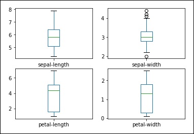
Box and Whisker Plots
You can create a histogram of each input variable to get an idea of the distribution using the commands shown below −
#histograms
dataset.hist()
plt().show()
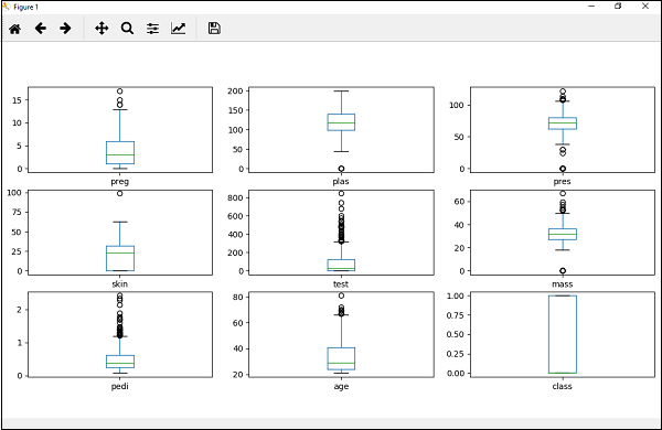
From the output, you can see that two of the input variables have a Gaussian distribution. Thus these plots help in giving an idea about the algorithms that we can use in our program.
Multivariate Plots
Multivariate plots help us to understand the interactions between the variables.
Scatter Plot Matrix
First, lets look at scatterplots of all pairs of attributes. This can be helpful to spot structured relationships between input variables.
from pandas.plotting import scatter_matrix
scatter_matrix(dataset)
plt.show()
You can observe the output as shown −
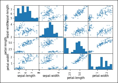
Observe that in the output there is a diagonal grouping of some pairs of attributes. This indicates a high correlation and a predictable relationship.
