
Article Categories
- All Categories
-
 Data Structure
-
 Networking
-
 RDBMS
RDBMS
-
 Operating System
-
 Java
Java
-
 MS Excel
-
 iOS
iOS
-
 HTML
HTML
-
 CSS
CSS
-
 Android
-
 Python
-
 C Programming
-
 C++
C++
-
 C#
C#
-
 MongoDB
-
 MySQL
MySQL
-
 Javascript
-
 PHP
PHP
-
 Economics & Finance
How to Rank data in reverse order in excel?
In this article, users will learn how to rank data in reverse order in Excel. Users may quickly identify the top performers or the data points with the highest values inside a dataset by giving lower ranks to higher values. When analyzing measures like sales numbers, performance indicators, or standings in various contests, this is especially helpful. Reverse-ranking the data makes it simple to compare the results to benchmarks or goals. Greater performance in comparison to other data points in the dataset is indicated by data points with higher ranks, which makes it easier to gauge success or progress using specified standards.
Example 1: To find Rank Data in Reverse Order in a Sheet
Step 1
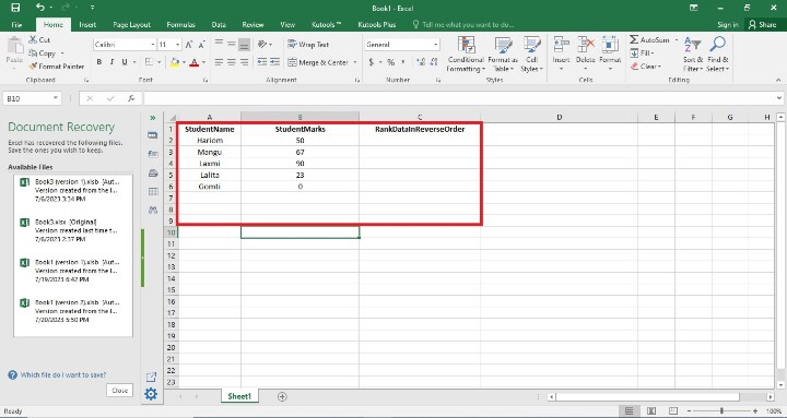
In the first step, users create the three columns in the worksheet i.e. StudentName, StudentMarksA, and RankdDataInReverseOrder Column. The RankDataInReverseOrder Column holds the data of rank in reverse order. Following is the screenshot of this step.
Step 2
In the step, users are entering the formula in the C2 Cell i.e. =RANK(B2,$B2:$B$6,1). Following is the screenshot of this step.
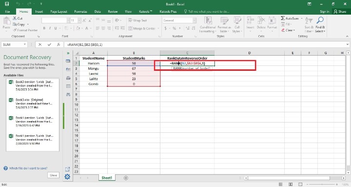
Explanation
=RANK(B2,$B2:$B$6,1)
Excel's RANK function is used in the formula provided to order the value in cell B2 about a range of values in column B. Let's investigate the formula:
The value you want to rank is represented by B2 in the current cell (where the formula is applied).
The range of values in column B that you want to compare against is denoted by $B$2:$B$6. When users replicate a formula to additional cells, the range stays fixed since the dollar signs ($) denote absolute cell references.
The RANK function's third input, 1, indicates that the rankings must be in decreasing order. Higher values will therefore be ranked lower.
This formula's goal is to rank the value in B2 in relation to all other values in the B2-B6 range. The value in B2 will be ranked as a consequence, with the greatest value having the lowest rank.
Step 3
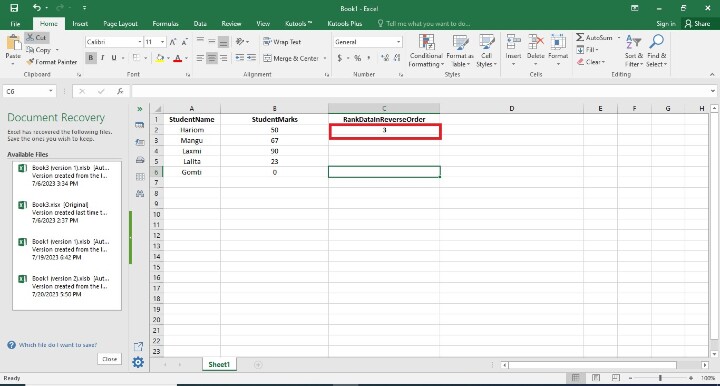
To find the rank of the RankDataInReverseOrder Column, press Enter. The cell will display the ranking. Following is the screenshot of this step.
Step 4
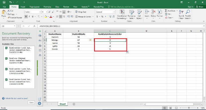
In this step, users find the remaining RankDataInReverseOrder cells by dragging the fill handle to the final cell where the user wants the rankings to appear (it's a tiny square in the bottom-right area of that row). In this step, the user has to see the result in reverse order. Following is the screenshot of this step.
Conclusion
When analyzing measurements or rankings where greater numbers denote superior performance, this is especially helpful. Reverse ranking also makes it simple to compare results to benchmarks or goals. The evaluation of progress or success in comparison to preset standards is made easier by looking at data points with lower rankings, which implies a greater performance relative to other data points in the dataset.

4K+ Views
