
Article Categories
- All Categories
-
 Data Structure
-
 Networking
-
 RDBMS
RDBMS
-
 Operating System
-
 Java
Java
-
 MS Excel
-
 iOS
iOS
-
 HTML
HTML
-
 CSS
CSS
-
 Android
-
 Python
-
 C Programming
-
 C++
C++
-
 C#
C#
-
 MongoDB
-
 MySQL
MySQL
-
 Javascript
-
 PHP
PHP
-
 Economics & Finance
How to Rank Data with multiple reference in excel?
Assigning ranks to data points based on their values under particular criteria or conditions is the aim of ranking data with multiple references in Excel. By using numerous references, users can tailor the ranking procedure to take into account various sets of information or circumstances, producing more precise and nuanced rankings. This enables users to customize the ranking process to match specific analysis requirements by assigning rankings based on various parameters, such as multiple columns, particular ranges, or complex circumstances.
When ranking data with numerous references, different data dimensions or features can be taken into account, allowing for a more thorough examination. This method enables users to consider several variables at once, giving us a more comprehensive picture and capturing the complexity of the dataset.
Example 1: To Find Rank Data with Multiple References in Excel
Step 1
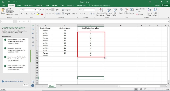
In the first step, users create the three columns in the worksheet i.e. Student Name, Student Marks, and Rank Data Column. The Rank Data Column holds the rank result. Here users are creating the data with multiple duplicate data in Student Name Field. Following is the screenshot of this step.

Step 2
In the step, users are entering the formula in the C2 cell i.e. =1+SUMPRODUCT(($A$2:$A$12=A2)*($B$2:$B$12>B2)). Following is the screenshot of this step.

Explanation
Users can use the formula you gave,1+SUMPRODUCT(($A$2:$A$12=A2)*($B$2:$B$12>B2)), to determine a rank or position in Excel based on particular criteria. Let's examine the formula in detail:
The range of cells in column A that we are contrasting against the value in cell A2 is represented as $A$2:$A$12.
The formula =A2 gives an array of TRUE or FALSE values after comparing each cell in the range $A$2:$A$12 to the value in cell A2.
The range of columns in column B that you are comparing the value in cell B2 to is $B$2:$B$12.
Cell B2 gives an array of TRUE or FALSE values after comparing each cell in the range $B$2:$B$12 to the value in cell B2.
The two arrays are multiplied element-by-element by ($A$2:$A$12=A2)*($B$2:$B$12>B2) to produce an array with TRUE values when both requirements are met and FALSE values in all other cases.
The SUMPRODUCT function adds up the array's values, counting how many of them are TRUE.
The sum of TRUE values is increased by 1 using the formula 1+SUMPRODUCT(($A$2:$A$12=A2)*($B$2:$B$12>B2)). This is done to obtain the desired ranking where positions begin at 1 rather than 0.
This formula's goal is to rank or position a certain value in column A according to a set of requirements in column B. The formula adds one to the count of cells in column B that satisfy the requirements (matching value in column A and higher value in column B) to determine the rank.
Step 3
To find the rank of the Rank Data Column enter the formula that is mentioned in previous steps and press Enter. Following is the screenshot of this step.

Step 4
In this step, users find the remaining Rank Data cells by copying the formula in all the cells i.e. C3 and C12. Users may also accomplish this by dragging the fill handle to the final cell where the user wants the rankings to appear (it's a tiny square in the bottom-right area of that row). So here users will see rank with multiple references. Following is the screenshot of this step.
Conclusion
In conclusion, using Excel to rank data with numerous references offers a strong tool for allocating ranks based on specific criteria, carrying out in-depth studies, as well as gleaning specific insights from a dataset. By using a variety of references, users can modify the ranking procedure to take into account various sets of information or circumstances, producing rankings that are more precise and nuanced.

950 Views
