
Article Categories
- All Categories
-
 Data Structure
-
 Networking
-
 RDBMS
RDBMS
-
 Operating System
-
 Java
Java
-
 MS Excel
-
 iOS
iOS
-
 HTML
HTML
-
 CSS
CSS
-
 Android
-
 Python
-
 C Programming
-
 C++
C++
-
 C#
C#
-
 MongoDB
-
 MySQL
MySQL
-
 Javascript
-
 PHP
PHP
-
 Economics & Finance
How To Easily Rank List Without Ties In Excel?
When working with data in Excel, it is frequently required to rank values in order to determine the highest or lowest values or to produce a sorted list. However, one common issue is dealing with linked values, which occur when two or more values have the same rank. This may make the ranking process more difficult and time?consuming.
Fortunately, Excel offers a straightforward technique for ranking a list without ties, guaranteeing that each item is assigned a unique rating. In this lesson, we will walk you through the process of using Excel's built?in functions to accomplish this. Whether you are a novice or a seasoned Excel user, this tutorial will assist you in mastering the art of ranking lists without ties. By the end of this session, you will be able to securely rank your data in Excel without any tied values, improving the accuracy and efficiency of your research. So, let's get started and discover the full potential of Excel's ranking skills!
Easily Rank List Without
Here we will use the rank and COUNTIF formulas to get the first value, then use the autofill handle to complete the task. So let us see a simple process to know how you can easily rank lists without ties in Excel.
Step 1
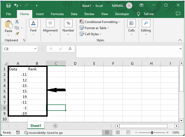
Consider an Excel sheet where you have scores with ties in them, similar to the below image.
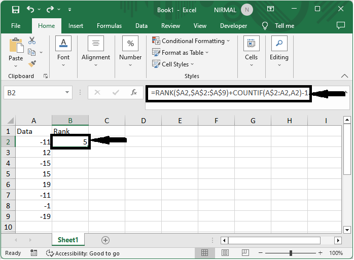
First, click on an empty cell and enter the formula as
=RANK($B2,$B$2:$B$9)+COUNTIF(B$2:B2,B2)?1 and click enter to get the first value's rank. In the formula B2:B9, the range of cells containing the scores
Empty cell > Formula > Enter.
Step 2
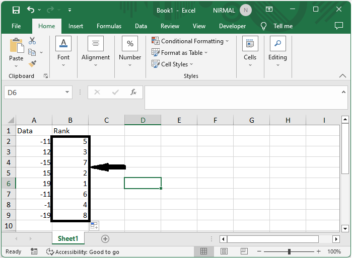
Then use the auto?fill handle to complete the task.
Conclusion
In this tutorial, we have used a simple example to demonstrate how you can easily rank lists without ties in Excel to highlight particular sets of data.

2K+ Views
