How to quickly color ranking in Excel?

In this article, the user will learn the process of coloring the cells in Excel based on the rank values. To do so, firstly user needs to evaluate the rank by using the provided rank formula, and after that obtained cells will be highlighted according to the user’s requirement. Another major benefit of learning this task is that analyzing data with the help of color is easier.

For example, consider that all the students who scored above 90 % marks will be displayed with green color. Then analyzing them from a large data set becomes an easy task. All this can be possible by using conditional formatting. It is a powerful feature of Excel, that allows user to automatically assigns different colors to values based on their ranks. Another effective way to visually highlight the ranking of data is by applying colors based on their ranks, as will be going to do in this task.

This task makes the data look more precise and experienced, by making the interpretation and analysis easy. This task allows the user to save lots of time while dealing with large datasets. The color coding helps allow users to easily rank the dataset by using the highest or lowest criteria.

Example 1: To color rank the cells in Excel by using the color formatting.

Step 1

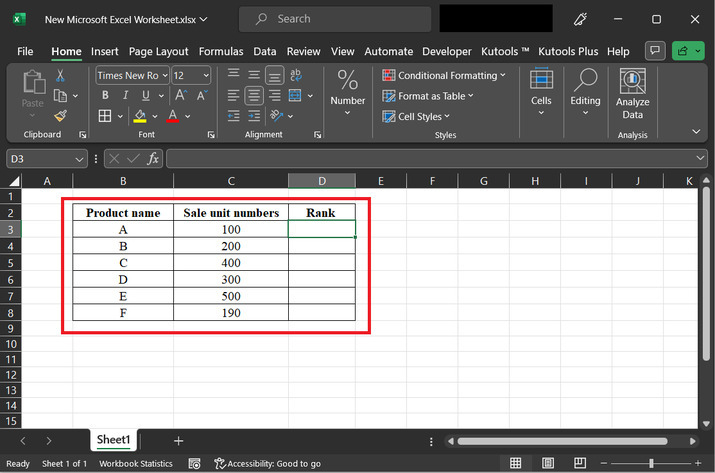
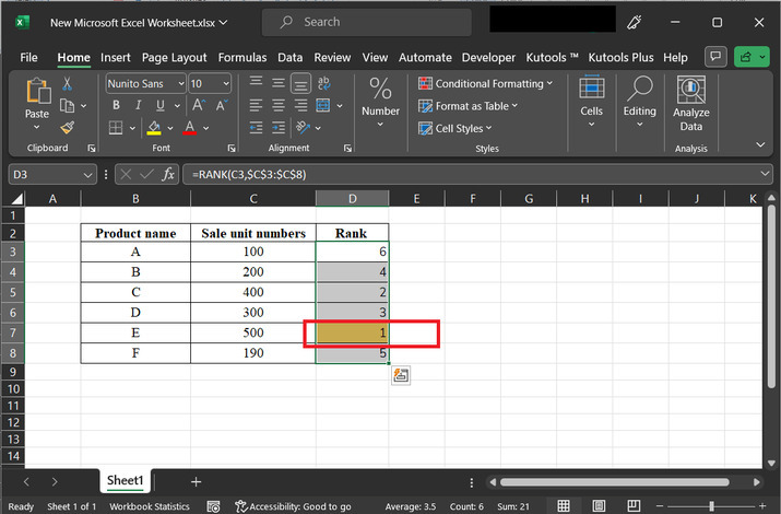
In this example, the user will learn the process of calculating the rank and after that will color the sheet accordingly. To begin with, the example, consider the first column with the name Product name, and second column with the name “Sale unit numbers”, and the third column with the name “Rank”. Consider the Excel spreadsheet provided below.

Step 2

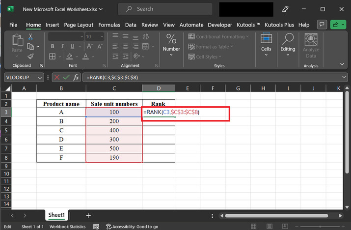
After that go to the D3 cell, and type formula “=RANK(C3,$C$3:$C$)”. This formula will allow the user to select the rank, for example, if there are two values 100, and 200. Then the greatest number will be provided with the highest rank, that is number 200 will have 1st rank. And number 100 will get 2^nd rank.

An explanation for the formula −

The formula "RANK (C3, $C$3:$C$)" is a function commonly used in spreadsheet software like Microsoft Excel or Google Sheets. It calculates the rank of a value within a given range of values. Here's a breakdown of the formula −

• "C3" represents the cell containing the value for which the user wants to determine the rank.

• "$C$3:$C$" represents the range of values in which you want to find the rank. The dollar signs ($) before the column and row references indicate that the reference is absolute.

The rank is determined as follows −

• The values in the range are sorted in descending order.

• The rank of the value in C3 is determined based on its position in the sorted list. The largest value obtains a rank of 1, the second largest obtains a rank of 2, and so on.

• For example, if the user has a list of numbers in the range C3:C10 and the user enters the formula "RANK (C3, $C$3:$C$10)" in cell D3, it will calculate the rank of the value in C3 among the values in C3:C10. The result will be a numerical value indicating the rank.

• This formula is useful for analyzing data and identifying the relative position of a value within a set of values. It can be used in various scenarios such as ranking sales figures, evaluating student scores, or assessing performance metrics.

Step 3

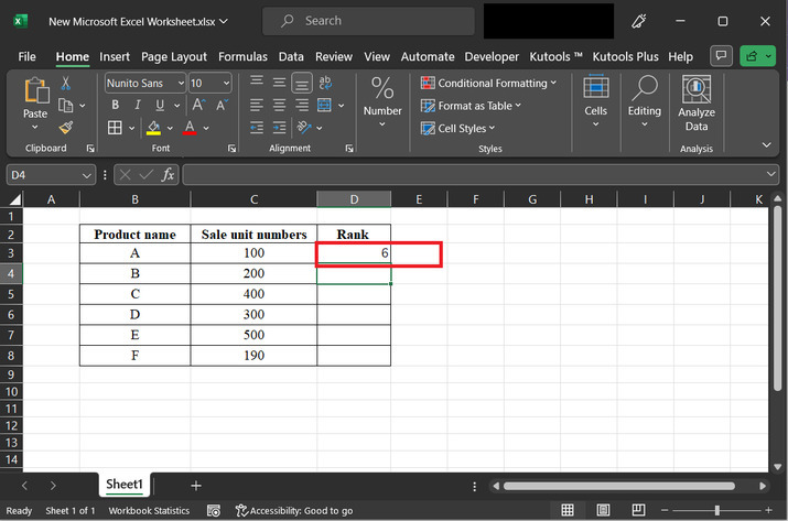
Press the “Enter” key and the result generated by the above step is provided in the below snapshot. Consider the below-provided snapshot for reference.

Step 4

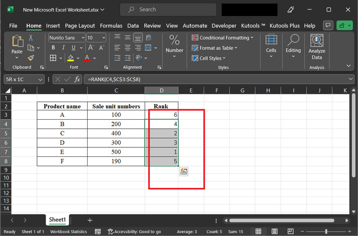
Drag the fill handle to copy the same results to another cell. The obtained results are depicted below −

Step 5

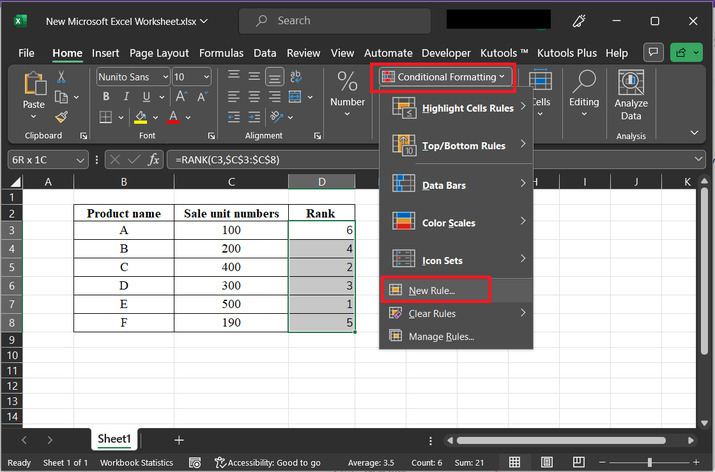
After solving the ranking, the user needs to focus on coloring the cells. To do so, click on the cell “Conditional Formatting”, and then select the option “New Rule”. Consider the below-depicted snapshot for code −

Step 6

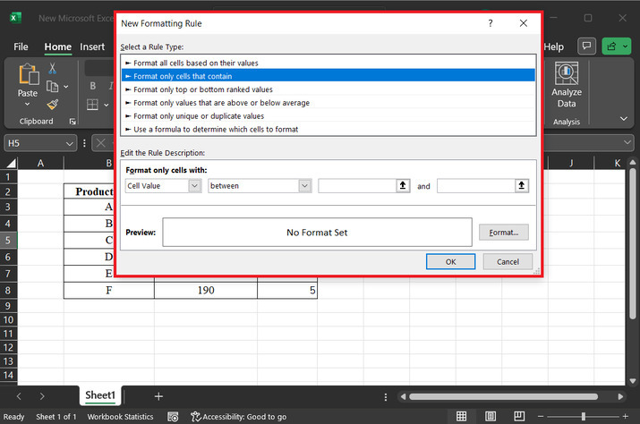
The above step will open a dialog box named “New Formatting Rule” which contains multiple options such as selecting a rule type, editing the rule description, and many others.

Step 7

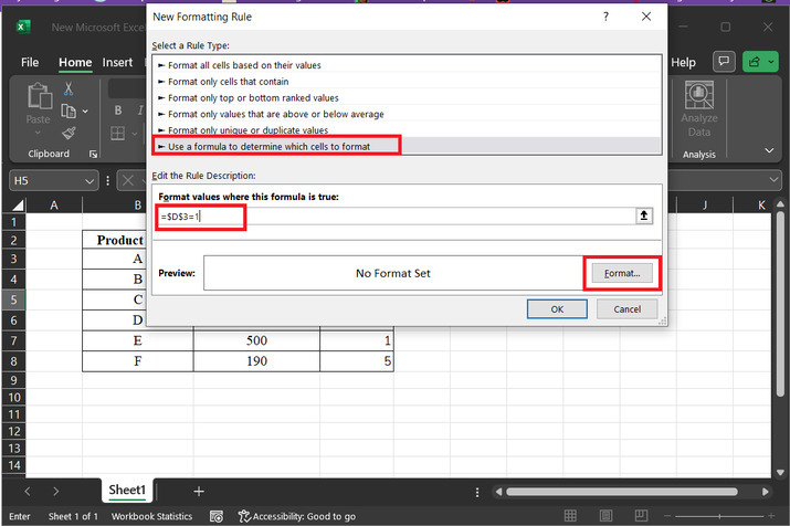
After that in the “select a rule type:” label, click on the “Use a formula to determine which cells to format” option, and in the “Edit the Rule Description” label type the formula “=$D$3=1”. Finally, click on the “Format” button. Consider the below-provided code snapshot −

Step 8

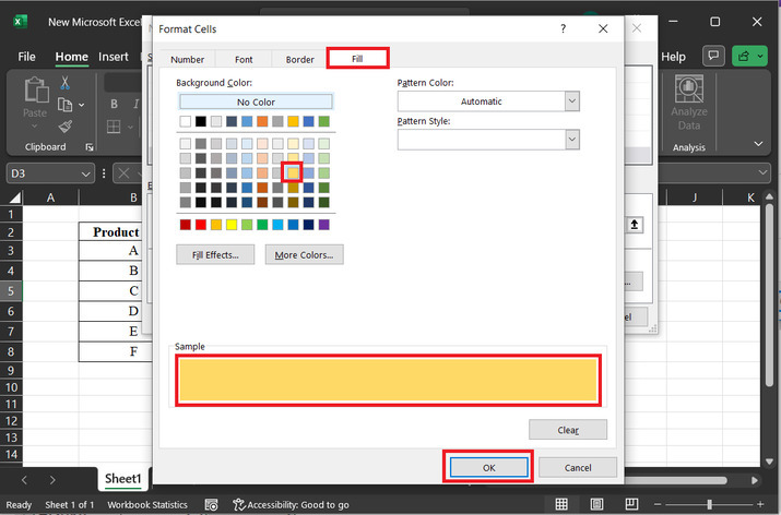
In the dialog box named “Format cells”, choose the tab named Fill. Choose any required color. Here, will be using the dark yellow color. After that click on the “OK” Button.

Step 9

Again, click on the “OK” button, and the cell that contains the rank value 1, will be highlighted automatically.

Please note that the user can repeat the last step for other ranks as well, and color can be chosen according to the user's requirement.

Conclusion

All the provided steps are clear, accurate, and precise. By referring to the provided steps user can easily able to highlight the ranked cells, according to its requirement.