
Article Categories
- All Categories
-
 Data Structure
-
 Networking
-
 RDBMS
RDBMS
-
 Operating System
-
 Java
Java
-
 MS Excel
-
 iOS
iOS
-
 HTML
HTML
-
 CSS
CSS
-
 Android
-
 Python
-
 C Programming
-
 C++
C++
-
 C#
C#
-
 MongoDB
-
 MySQL
MySQL
-
 Javascript
-
 PHP
PHP
-
 Economics & Finance
How to Create a Chart in Ranking Order in Excel?
Ranking charts let you display data in a way that emphasises the relative placements of various items or categories. Charts are a great tool for visualising data. Ranking charts can be a useful tool for comparing sales data, assessing performance, or analysing survey results.
In this article, we'll show you step-by-step how to create an Excel chart that ranks data. After sorting the data, we'll finish the work by making a bar chart. You will have a basic understanding of how to use Excel's features to construct ranking charts that are both aesthetically pleasing and educational by the end of this session. So let's get started and discover the power of Excel's ranking charts!
Create a Chart in Ranking Order
Here we will first sort the data in ascending or descending order, then create a bar chart to complete the task. So let us see a simple process to learn how you can create a chart in ranking order in Excel.
Step 1
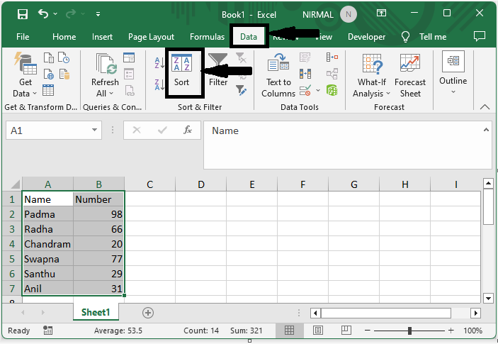
Consider an Excel sheet where you have required data to create chart.
First, select the range of cells, then click on Data and select Sort.
Select Cells > Data > Sort.
Step 2
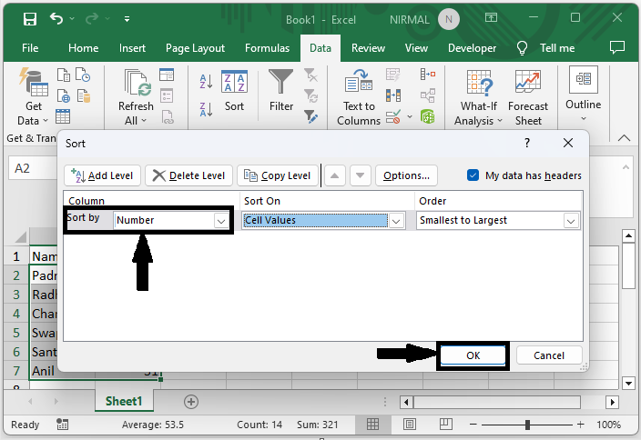
Then select column B, Sort on to values, and order from smallest to largest, and click Ok.
Column > Sort On > Order > Ok.
Step 3
Then select the range of cells, click on insert, and select Bar chart.
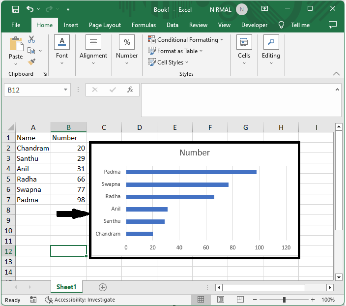
This is how you can create a chart in ranking order in Excel.
Conclusion
In this tutorial, we have used a simple example to demonstrate how you can create a chart in ranking order in Excel to highlight a particular set of data.

3K+ Views
