How to minimize or hide the Ribbon in Excel?

In the article, the users are going to hide or minimize the ribbon in Microsoft Excel. The users can right-click on the ribbon to minimize or hide all the tabs. This method may be completed utilizing an easy way within Microsoft Excel by using the Ku-tools tab to minimize the ribbon. The two examples are demonstrated in this article to hide the Ribbon in Excel. Multiple tabs are presented in ribbon to be used by the users to achieve the targeted goals. The step-by-step explanation is depicted in both examples to show a similar result.

Let us start with few examples.

Example 1: To minimize or hide the ribbon in Excel

Step 1

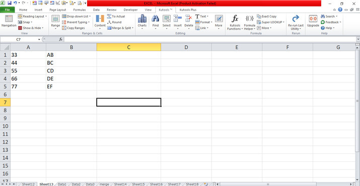
Deliberate the Excel worksheet. First, open the Excel sheet and create the data one by one from cells A1 to B5 in any cell according to the need.

Step 2

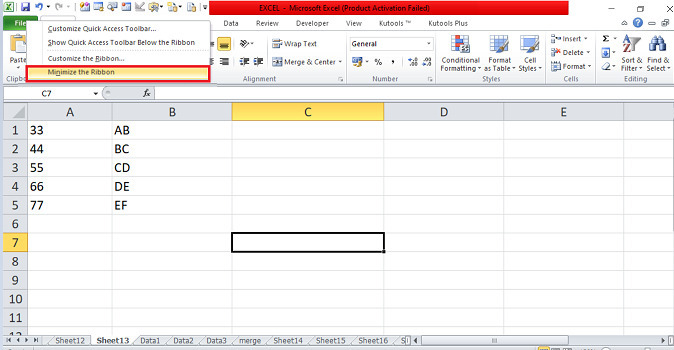
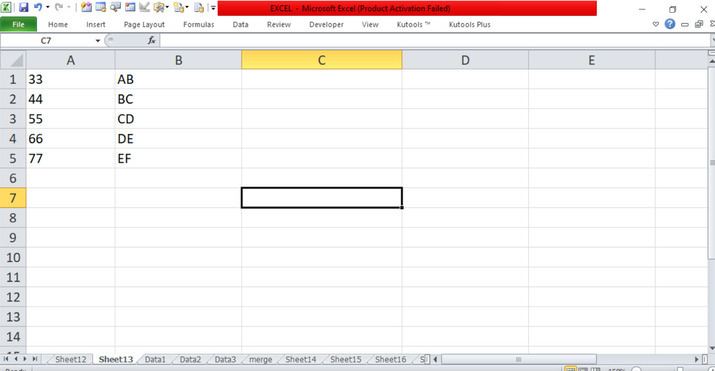
In the sheet, place the cursor in the ribbon. In the ribbon, there are many tabs included in the top corner. Place the cursor in the top corner of the ribbon and right-click on it. There are many options included in the menu. Place the cursor and click on the Minimize the ribbon tab which will minimize or hide the ribbon automatically as shown below.

Example 2: Minimize or hide the ribbon by using Ku-tools

Step 1

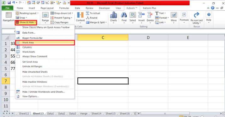
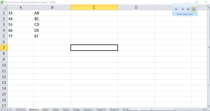
To minimize the ribbon, place the cursor in the ribbon. In the ribbon, there are many tabs included in the top corner. Place the cursor in the Ku-tools tab and click on the tab that has many options included. On the Ku-tools tab, place the cursor and click on the Show & Hide tab which has a drop-down menu on the Ranges & Cells group. Click on the menu and select the Work Area tab which will open the pane in the right corner as shown below.

Step 2

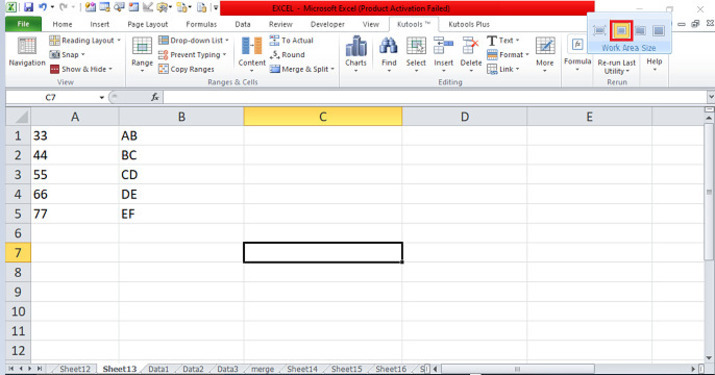
In the sheet, place the cursor in the pane and select the first Work Area size in the corner. After clicking on it, it will minimize the ribbon as well as the status bar as shown below.

Step 3

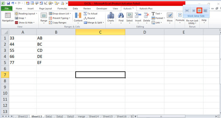
In the sheet, place the cursor in the pane and select the second Work Area size in the corner. After clicking on it, it will minimize the ribbon as well as the formula bar and status bar as shown below.

Step 4

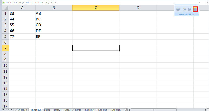
In the sheet, place the cursor in the pane and select the third Work Area size in the corner. After clicking on it, it will hide or minimize the ribbon as well as the formula bar and status bar and it may also hide the ribbon as shown below.

The users utilized the easy instances to display how they hide or minimize the area of the ribbon by using right-clicking on the ribbon in the top corner and using the Ku-tools tab which the work area is included on it. The users used the necessary tabs which are included in the ribbon. They have to practice the essential options from the ribbon and modify the data according to the need.