How to hide every other row in Excel?

Hiding data simply means making the view of data unavailable for the user. This can be done either to hide the confidential data or to hide the unnecessary or scrap data to make the sheet look clearer and more precise. This article guides users with two different strategies to achieve the same task. The first approach uses VBA code to implement the required functionality while the second approach is based on the use of Kutools. All the steps are precisely and thoroughly provided with the help of proper snapshots.

Example 1: To hide the rows within the Excel by using the VBA code

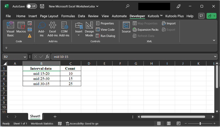
Step 1

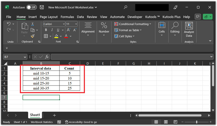
To understand the process of hiding the rows, by using the VBA code. Consider the below given excel spreadsheet. This spreadsheet contains two column, among them first column specifies the interval while the second column will calculate the count for each provided interval.

Step 2

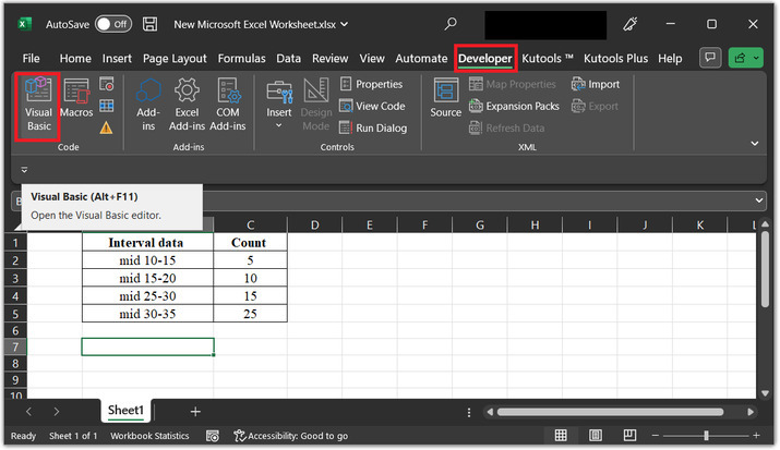
To run the VBA code, user need to open the VBA code area, to do so, click on the “developer” option, then choose “Visual Basic” option, under the code section.

Step 3

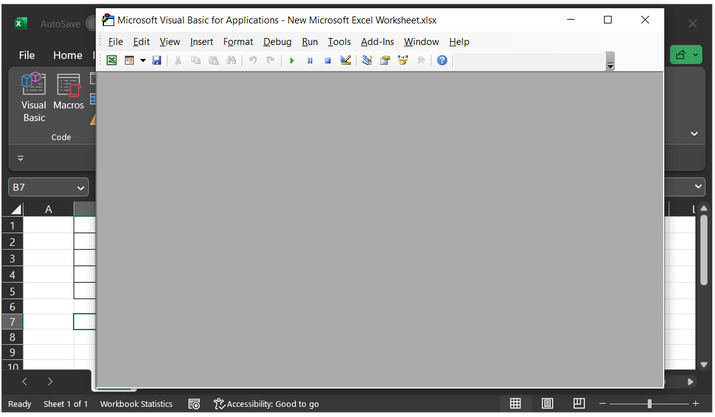
The above step will open a “Microsoft Visual Basic for Applications” dialog box, as specified above.

Step 4

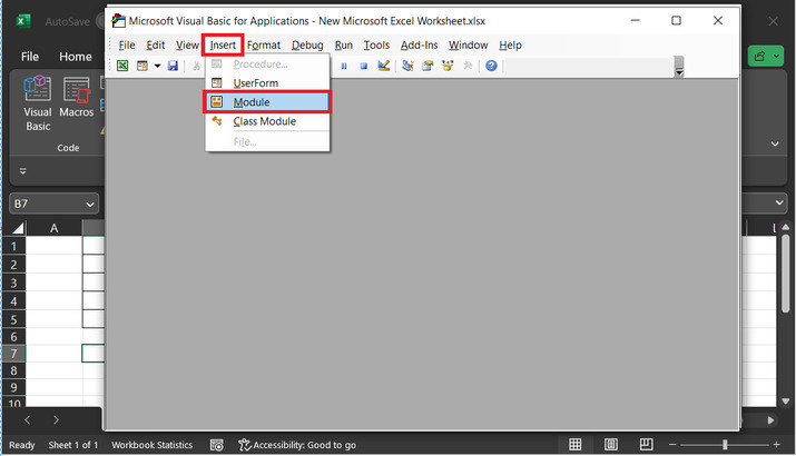
In the available list of options click on the “Insert” tab, and then choose the option for “module”.

Step 5

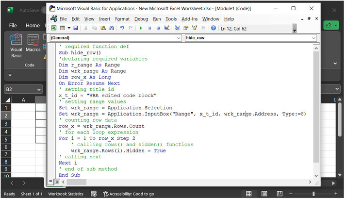
The above step will open a code area. In the opened code area, copy the below-provided code −

' required function def
Sub hide_row()
'declaring required variables
Dim r_range As Range
Dim wrk_range As Range
Dim row_x As Long
On Error Resume Next
' setting title id
x_t_id = "VBA edited code block"
' setting range values
Set wrk_range = Application.Selection
Set wrk_range = Application.InputBox("Range", x_t_id, wrk_range.Address, Type:=8)
' counting row data
row_x = wrk_range.Rows.Count
' for each loop expression
For i = 1 To row_x Step 2
   ' callling rows() and hidden() functions
   wrk_range.Rows(i).Hidden = True
' calling next
Next i
' end of sub method
End Sub

Please use proper code indentation to avoid possible code errors.

Code snapshot

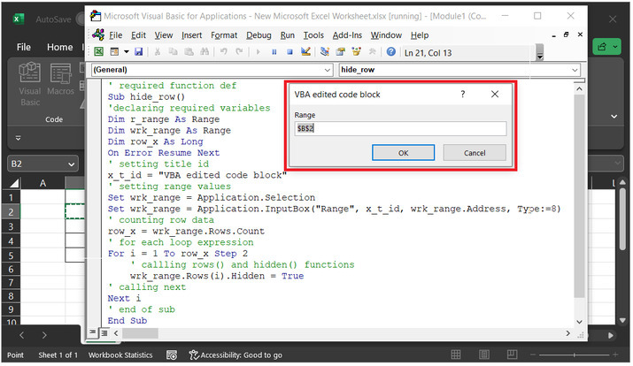
Step 6

Run the above code by using the “F5” key. This will display a new dialog box, with the heading “VBA edited code block”, as specified within the coding expressions. In the newly open window enter the cell or row value the user wants to hide, for this example will take B2 cell data. Consider below given snapshot for data −

Step 7

Press “Alt+Q” to hide 2nd-row data. Consider the below-provided output snapshot, their user will understand that the second-row data will become hidden, and can be seen by double-clicking on the row header provided in the worksheet.

Example 2: To hide the rows within the Excel by using the Kutools

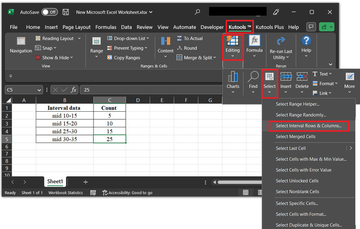
Step 1

Consider the same worksheet, as used in the above example. This example will perform the same task by using the kutools. Open the “Kutools” tab, and click on the “Editing” section. In the “editing section” select the option “Select”. In the drop-down options list of select sections select “Select Intervals Rows and Columns...”. Consider the below-given image for proper reference −

Step 2

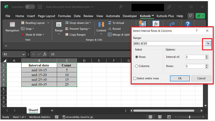
The above step will open the “Select Interval Rows & Columns” dialog box. In the opened dialog box, click on the below highlight button. This button will allow the user to select the required data values from the sheet.

Step 3

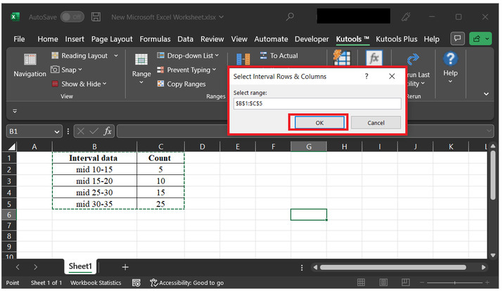
For this example, will assume the range as B1 to C5. Consider below highlighted image for reference. Click on the “OK” button.

Step 4

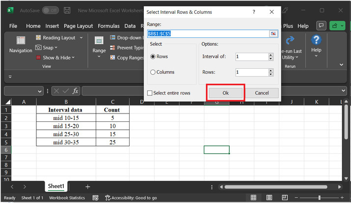
The above step will display the selected cell range inside the range label. In the select label, choose the option “Rows”, enter 1 in the “Interval of” data. Finally, click on “Ok” button.

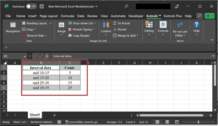
Step 5

The above step will select the table rows alternatively, as depicted below −

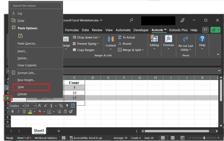
Step 6

Right on the number label provided at the left hand side of the sheet, and click on the “hide” option.

Step 7

This will hide the selected rows. Consider below given image for reference −

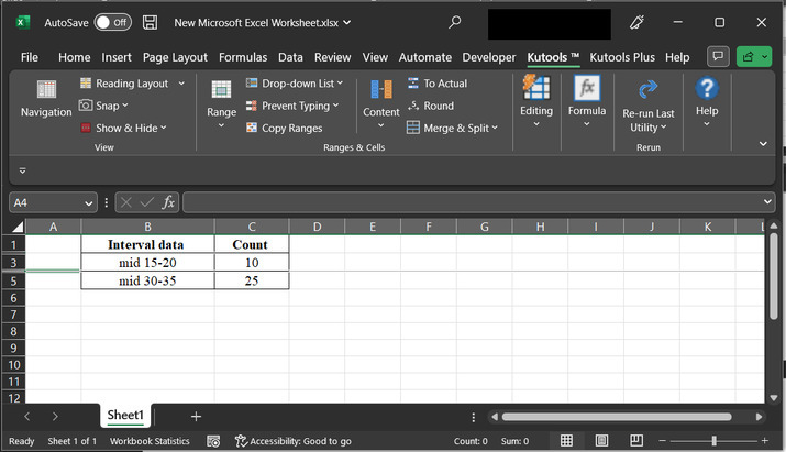
Please note that users can view the hidden rows by clicking on the row header.

Conclusion

In this article, learners will understand the stepwise explanation for the task of “hiding row” by using two simple approaches. Here, the first approach is based on the method of using the VBA Code, while the second method is based on the process of using the Kutools. Both the provided task will generate the same result, the only difference between them is the way of implementation.