How to hide negative numbers in Excel?

In Excel, the user will understand the concept of how to hide negative numbers in Excel. Equations can also be written using integers with negative values. In this article, the user will learn three common examples. The first example is based on negative numbers by using conditional formatting. The second example is based on hiding the negative number by using the format cell option. Both examples are explained thoroughly within the article.

Example 1: To hide the negative numbers in Excel by using the conditional formatting

Step 1

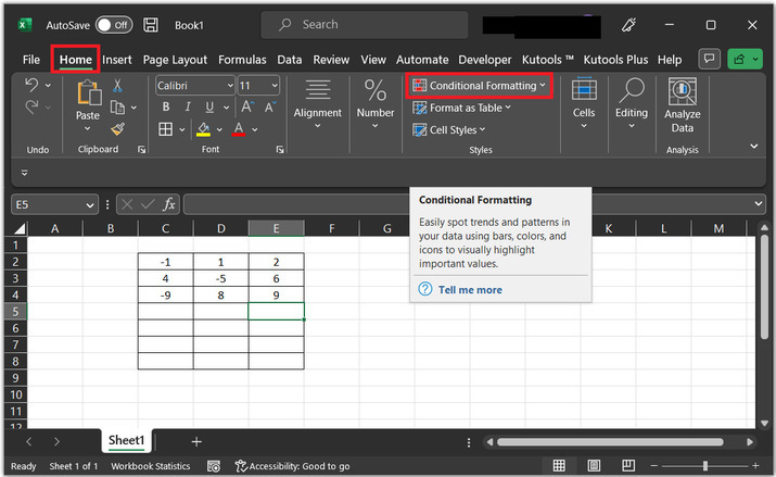
The sample spreadsheet contains total 9 numbers. Few of them are negative values. To start the article, select the data which is highlighted in below image.

Step 2

Go to the Home Tab under the Styles group and select the Conditional Formatting arrow as highlighted below image −

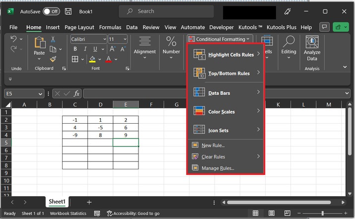
Step 3

After select the conditional formatting’s drop menu. a menu list will appear as highlighted in the below image −

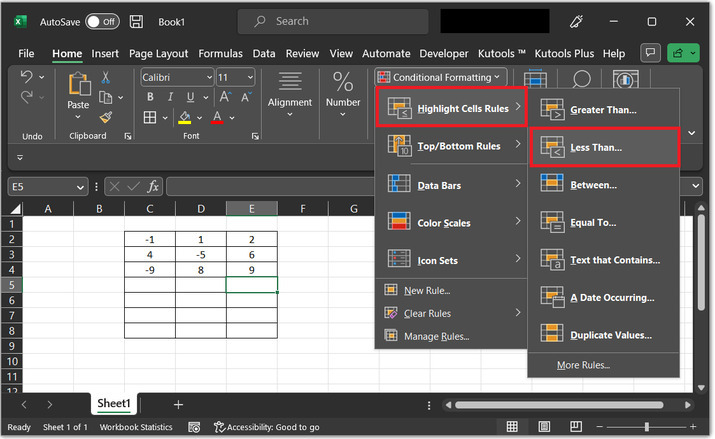
Step 4

Click on the Highlight Cells Rules arrow and then select Less Than… option, to highlight the below image.

Step 5

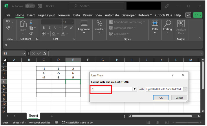
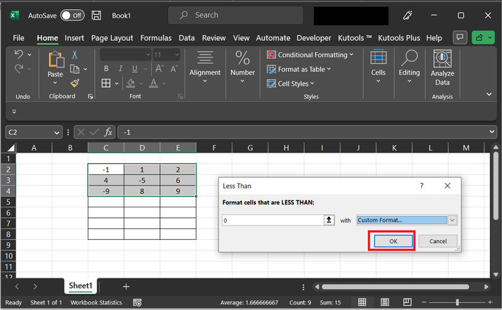
After clicking on the Less Than… option a Less Than dialog box appears on the sheet. Consider below provided snapshot −

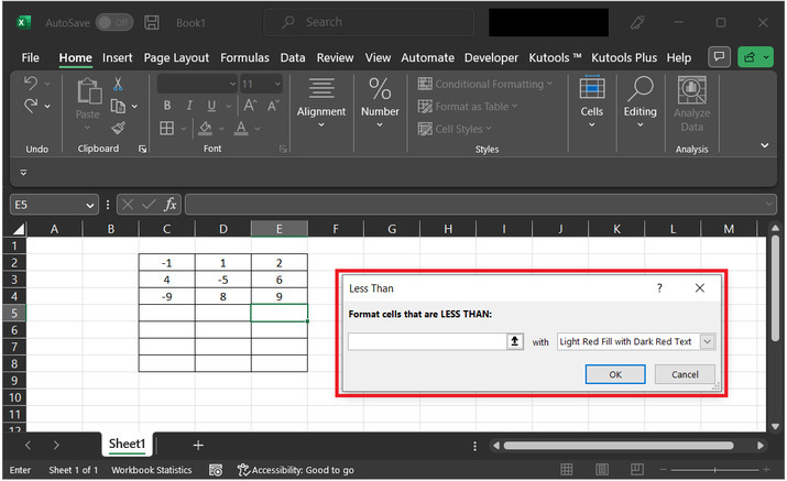
Step 6

In Format cells that are LESS THAN: text box enter 0.

Step 7

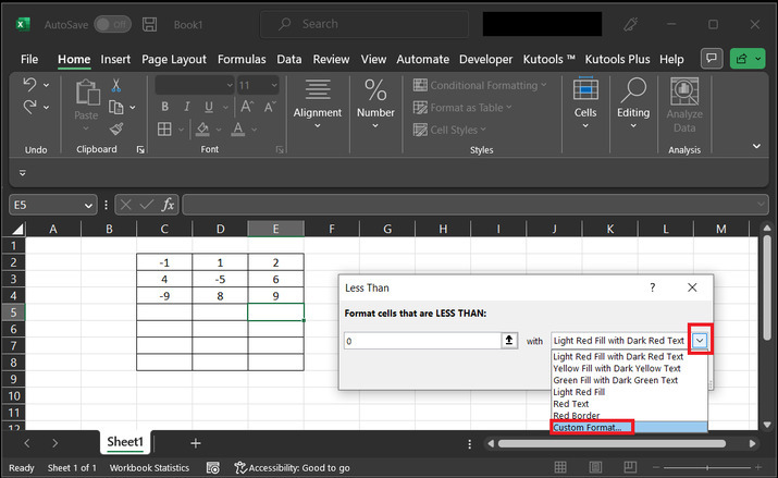
Now press the drop down arrow provided on the side of the “with” text box and select Custom Format..

Step 8

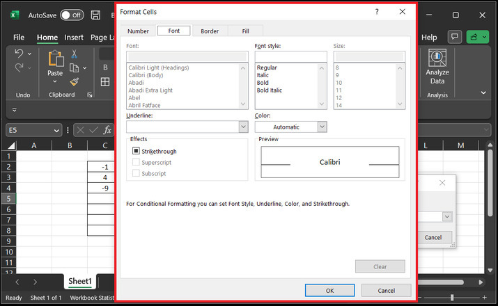
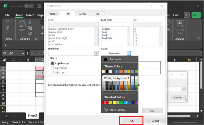
This will open a Format cells dialog box. This dialog box, comprises four tabs as display in the below image −

Step 9

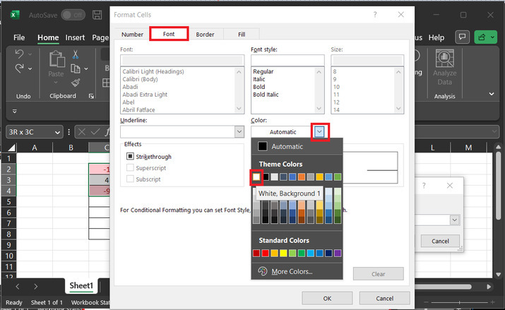
To perform the required task, choose the Font Tab and in Color section opt for white color, this will modify the font color of negative number to white, and the numbers can become invisible on work sheet.

Step 10

Now select the OK button that will close the dialog box named Format Cells.

Step 11

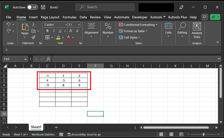
Again, select the highlighted button named OK“Less than” dialog box.

Consider the final provided output snapshot below. All the negative values are now become invisible due to the use of white color font.

Example 2: To hide the negative numbers in Excel by using the format cell option

Step 1

Again, consider the same worksheet. Firstly select the cell range by using the negative numbers. Consider the below image for reference −

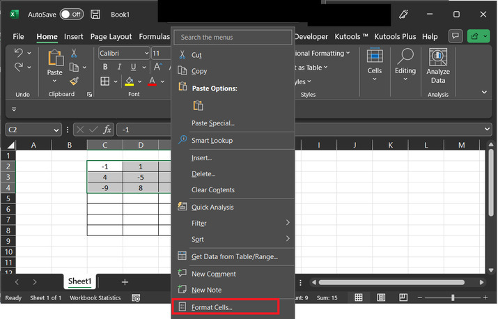
Step 2

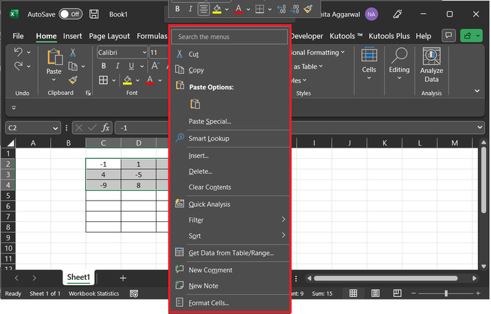
Now right-click on the selected range. This will display a drop-down menu on the right-hand side of the selected cells.

Step 3

From the list of appeared option, select “Format Cells…”.

Step 4

This will finally, display a “Format Cells” dialog box. This dialog box, contains many option tabs such as numbers, alignment, and many other.

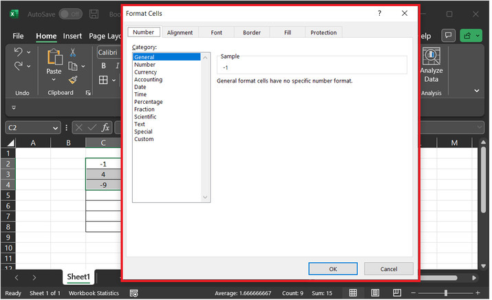
Step 5

Go to the Number Tab, and from the Category section select the “Custom” option.

Step 6

Move to the “Type:” section and in the provided textbox enter “0; ”. To extract all the negative values, that is number less than 0.

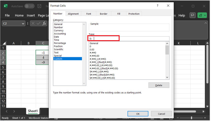
Step 7

Now in the dialog box named Format Cells, close this dialog box by pressing the OK button.

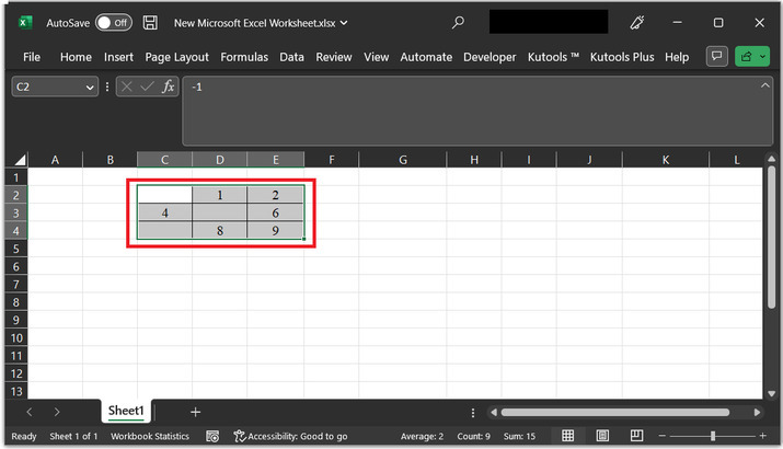
Step 8

The above step will replace all the negative values with space. Consider below provided screenshot for proper reference −

Example 3: To hide the negative numbers in Excel by using the kutools

Step 1

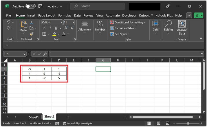
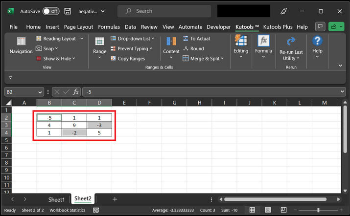
Consider the below given worksheet. This worksheet contains 9 entries numeric entries.

Step 2

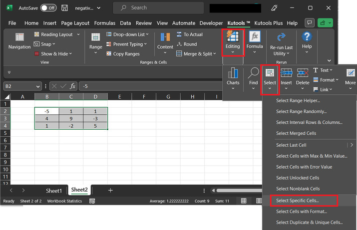
After that go to the “Kutool” option, and choose “Editing” option. Further, choose the “Select” option from the editing section, and click on “Select Specific Cells…”.

Step 3

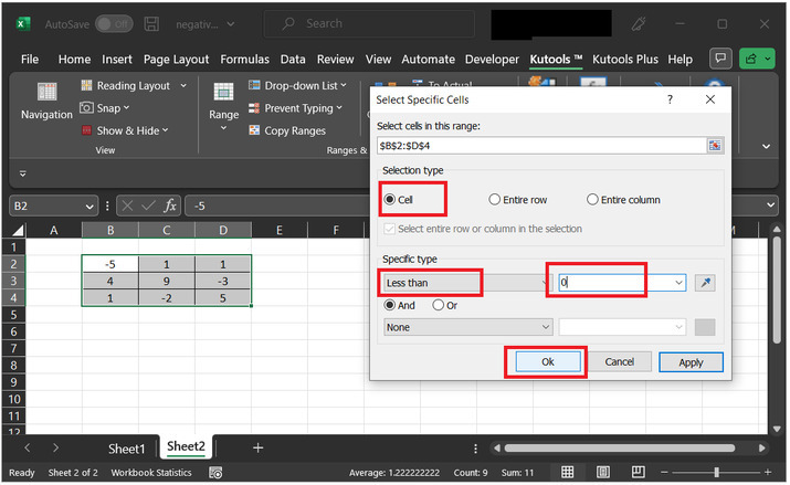
The above step will open a “Select Specific Cells” dialog box. In this dialog box, select the first option “Cell”, and under the specific type option, choose “Less than” In the next input value box, enter “0”. Finally, click on the “OK” button.

Step 4

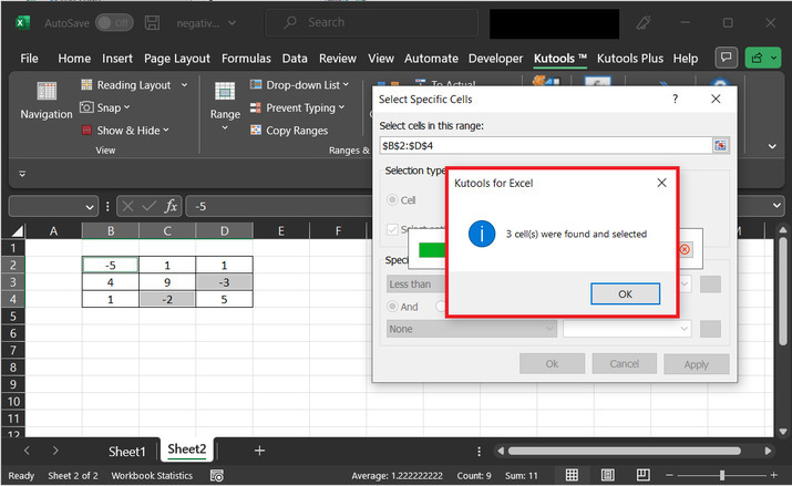
The new dialog box would be opened, with heading “Kutool for excel”. Click on “OK”. This will select all the cells with negative values.

Step 5

Consider snapshot of selected data cells −

Step 6

Again select the “Home” tab, and under the “Font” section, select the last option, and select the “White” color as provided below −

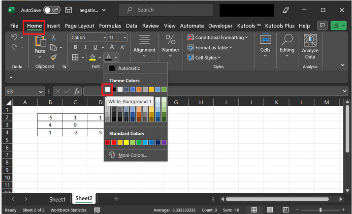
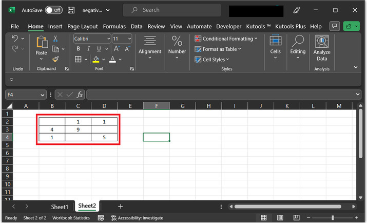
Step 7

This step will hide all the negative values by changing their font to white color.

Conclusion

This article focusses on guiding about the three different ways, by using which use can hide the negative numbers in excel. All the provided stepwise data explanation is accurate and precise. In the first example, the conditional formatting would be used to resolve the given problem statement. Format cell option is used in the second example. Kutools option is depicted in the third example to hide the negative number.