How to change/edit Pivot Chart's data source/axis/legends in Excel?

Excel's Pivot Chart does not allow users to modify the data source it uses. Having said that, you may come across situations where you will need to alter the data source of a pivot chart. This tutorial will show you how to alter the data source of a pivot chart in Excel, as well as how to edit the axis labels and legends of a pivot chart in Excel.

Changing a Pivot Chart’s Axis/Legends in Excel

Within Excel's Filed List, altering or editing the Pivot Chart's axis and legends is actually fairly straightforward and simple to do. You also have the following options.

Let’s understand step by step with an example.

Step 1

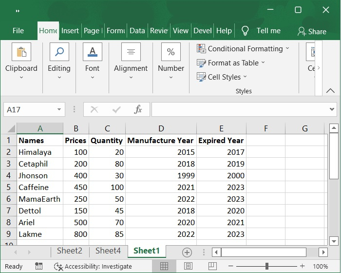
Let’s assume we have a sample data for creating pivot chart, as shown in the following screenshot.

Step 2

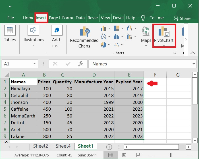
Now, select the data range from A1:E9. Click on the Insert tab on the tool bar ribbon and then select PivotChart option to insert pivot chart for selected data range. Refer to the below screenshot for the same.

Step 3

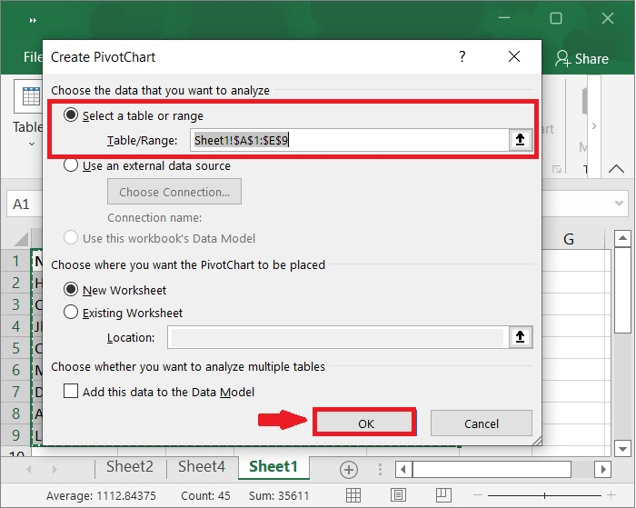
In the next step, create Pivot chart window appears, make sure the data range is selected as A1:E9 under Select a table or range option. Now, choose new worksheet to create the pivot chart in separate sheet then click on OK button. Check out the below screenshot below.

Step 4

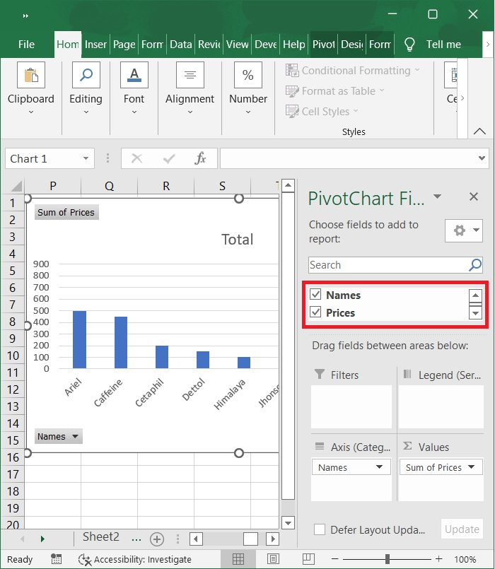
The pivot chart is now created in a separate worksheet. In the pivot chart fields check Names and Prices. After those values appear refer to the below screenshot for the same.

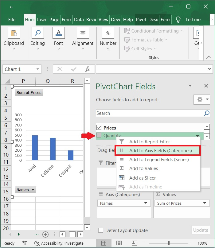
Step 5

In the next step, in order to add another axis, right click on any field from the list and select “Add to Axis Field” from the below screenshot you can check we have selected Quantity filed to add to axis field.

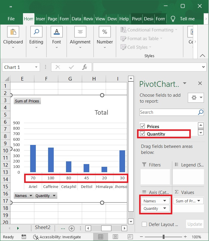
Step 6

Now, the quantity field is added in our pivot chart and it’s moved under Axis category list. Refer to below screenshot for the same.

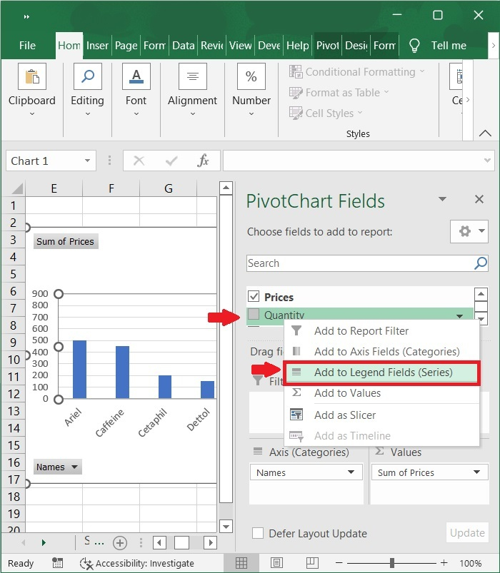
Step 7

To add/show filed as Legends, right click on any field from the list and select “Add to Legend Field” from the below screenshot you can check we have selected Quantity filed to add to legend fields.

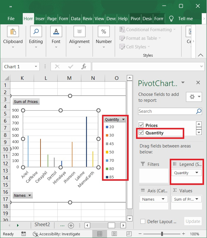
Step 8

Now, the quantity field is added in our pivot chart and it’s moved under Legends category list. A separate legend view is displayed on the pivot chart showing a unique color for each quantity. Refer to below screenshot for the same.

Changing a Pivot Chart’s Data Source in Excel

In the following steps, we will explain how you can change/edit a pivot chart's data source in Excel.

Step 9

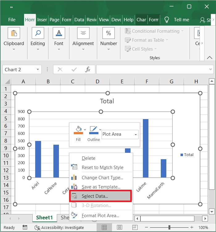
To change the data source of a pivot chart, copy the pivot and paste it in a separate excel workbook. Now, highlight the graph area and right click on the graph to display the options, then choose select data from the list. Refer to the below screenshot for the same.

Step 10

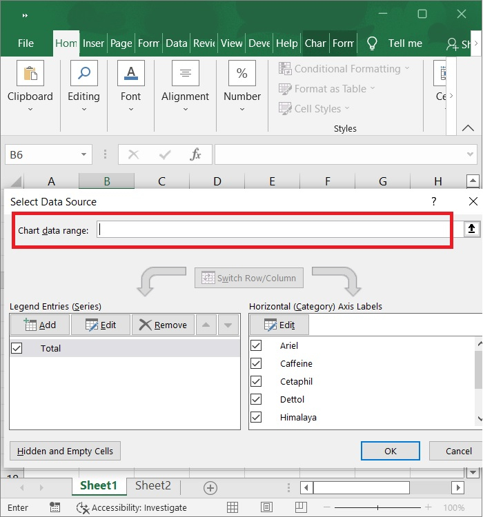
Select Data source window is displayed now, choose the data range to replace the chart data with the new data as shown in the below screenshot.

Step 11

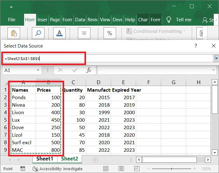
Select the data range for modifying the chart data, here we have chosen data range from A1:B9. Refer to the below screenshot for the same.

Step 12

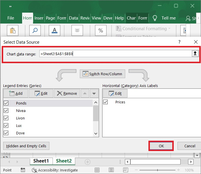
After selecting the data range, the selected data range is shown under the chart data range box. Make sure the new data is selected and then, click Ok to replace the data source. Check out the screenshot below.

Step 13

Now, the chart data is updated with the new selected data. Below is the screenshot for the same.

Conclusion

In this tutorial, we explained in a step‑by‑step manner how you can edit or change a pivot chart's axis, legends and how to replace the data source.