- DSP - Home
- DSP - Signals-Definition
- DSP - Basic CT Signals
- DSP - Basic DT Signals
- DSP - Classification of CT Signals
- DSP - Classification of DT Signals
- DSP - Miscellaneous Signals
- Operations Signals - Shifting
- Operations Signals - Scaling
- Operations Signals - Reversal
- Operations Signals - Differentiation
- Operations Signals - Integration
- Operations Signals - Convolution
- Basic System Properties
- DSP - Static Systems
- DSP - Dynamic Systems
- DSP - Causal Systems
- DSP - Non-Causal Systems
- DSP - Anti-Causal Systems
- DSP - Linear Systems
- DSP - Non-Linear Systems
- DSP - Time-Invariant Systems
- DSP - Time-Variant Systems
- DSP - Stable Systems
- DSP - Unstable Systems
- DSP - Solved Examples
- Z-Transform
- Z-Transform - Introduction
- Z-Transform - Properties
- Z-Transform - Existence
- Z-Transform - Inverse
- Z-Transform - Solved Examples
- Discrete Fourier Transform
- DFT - Introduction
- DFT - Time Frequency Transform
- DTF - Circular Convolution
- DFT - Linear Filtering
- DFT - Sectional Convolution
- DFT - Discrete Cosine Transform
- DFT - Solved Examples
- Fast Fourier Transform
- DSP - Fast Fourier Transform
- DSP - In-Place Computation
- DSP - Computer Aided Design
- Digital Signal Processing Resources
- DSP - Quick Guide
- DSP - Useful Resources
- DSP - Discussion
DSP - Operations on Signals Scaling
Scaling of a signal means, a constant is multiplied with the time or amplitude of the signal.
Time Scaling
If a constant is multiplied to the time axis then it is known as Time scaling. This can be mathematically represented as;
$x(t) \rightarrow y(t) = x(\alpha t)$ or $x(\frac{t}{\alpha})$; where α ≠ 0
So the y-axis being same, the x- axis magnitude decreases or increases according to the sign of the constant (whether positive or negative). Therefore, scaling can also be divided into two categories as discussed below.
Time Compression
Whenever alpha is greater than zero, the signals amplitude gets divided by alpha whereas the value of the Y-axis remains the same. This is known as Time Compression.
Example
Let us consider a signal x(t), which is shown as in figure below. Let us take the value of alpha as 2. So, y(t) will be x(2t), which is illustrated in the given figure.
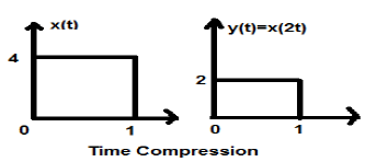
Clearly, we can see from the above figures that the time magnitude in y-axis remains the same but the amplitude in x-axis reduces from 4 to 2. Therefore, it is a case of Time Compression.
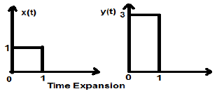
Time Expansion
When the time is divided by the constant alpha, the Y-axis magnitude of the signal get multiplied alpha times, keeping X-axis magnitude as it is. Therefore, this is called Time expansion type signal.
Example
Let us consider a square signal x(t), of magnitude 1. When we time scaled it by a constant 3, such that $x(t) \rightarrow y(t) \rightarrow x(\frac{t}{3})$, then the signals amplitude gets modified by 3 times which is shown in the figure below.
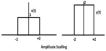
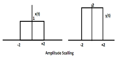
Amplitude Scaling
Multiplication of a constant with the amplitude of the signal causes amplitude scaling. Depending upon the sign of the constant, it may be either amplitude scaling or attenuation. Let us consider a square wave signal x(t) = Π(t/4).
Suppose we define another function y(t) = 2 Π(t/4). In this case, value of y-axis will be doubled, keeping the time axis value as it is. The is illustrated in the figure given below.
Consider another square wave function defined as z(t) where z(t) = 0.5 Π(t/4). Here, amplitude of the function z(t) will be half of that of x(t) i.e. time axis remaining same, amplitude axis will be halved. This is illustrated by the figure given below.