- Signals & Systems Home
- Signals & Systems Overview
- Introduction
- Signals Basic Types
- Signals Classification
- Signals Basic Operations
- Systems Classification
- Types of Signals
- Representation of a Discrete Time Signal
- Continuous-Time Vs Discrete-Time Sinusoidal Signal
- Even and Odd Signals
- Properties of Even and Odd Signals
- Periodic and Aperiodic Signals
- Unit Step Signal
- Unit Ramp Signal
- Unit Parabolic Signal
- Energy Spectral Density
- Unit Impulse Signal
- Power Spectral Density
- Properties of Discrete Time Unit Impulse Signal
- Real and Complex Exponential Signals
- Addition and Subtraction of Signals
- Amplitude Scaling of Signals
- Multiplication of Signals
- Time Scaling of Signals
- Time Shifting Operation on Signals
- Time Reversal Operation on Signals
- Even and Odd Components of a Signal
- Energy and Power Signals
- Power of an Energy Signal over Infinite Time
- Energy of a Power Signal over Infinite Time
- Causal, Non-Causal, and Anti-Causal Signals
- Rectangular, Triangular, Signum, Sinc, and Gaussian Functions
- Signals Analysis
- Types of Systems
- What is a Linear System?
- Time Variant and Time-Invariant Systems
- Linear and Non-Linear Systems
- Static and Dynamic System
- Causal and Non-Causal System
- Stable and Unstable System
- Invertible and Non-Invertible Systems
- Linear Time-Invariant Systems
- Transfer Function of LTI System
- Properties of LTI Systems
- Response of LTI System
- Fourier Series
- Fourier Series
- Fourier Series Representation of Periodic Signals
- Fourier Series Types
- Trigonometric Fourier Series Coefficients
- Exponential Fourier Series Coefficients
- Complex Exponential Fourier Series
- Relation between Trigonometric & Exponential Fourier Series
- Fourier Series Properties
- Properties of Continuous-Time Fourier Series
- Time Differentiation and Integration Properties of Continuous-Time Fourier Series
- Time Shifting, Time Reversal, and Time Scaling Properties of Continuous-Time Fourier Series
- Linearity and Conjugation Property of Continuous-Time Fourier Series
- Multiplication or Modulation Property of Continuous-Time Fourier Series
- Convolution Property of Continuous-Time Fourier Series
- Convolution Property of Fourier Transform
- Parseval’s Theorem in Continuous Time Fourier Series
- Average Power Calculations of Periodic Functions Using Fourier Series
- GIBBS Phenomenon for Fourier Series
- Fourier Cosine Series
- Trigonometric Fourier Series
- Derivation of Fourier Transform from Fourier Series
- Difference between Fourier Series and Fourier Transform
- Wave Symmetry
- Even Symmetry
- Odd Symmetry
- Half Wave Symmetry
- Quarter Wave Symmetry
- Fourier Transform
- Fourier Transforms
- Fourier Transforms Properties
- Fourier Transform – Representation and Condition for Existence
- Properties of Continuous-Time Fourier Transform
- Table of Fourier Transform Pairs
- Linearity and Frequency Shifting Property of Fourier Transform
- Modulation Property of Fourier Transform
- Time-Shifting Property of Fourier Transform
- Time-Reversal Property of Fourier Transform
- Time Scaling Property of Fourier Transform
- Time Differentiation Property of Fourier Transform
- Time Integration Property of Fourier Transform
- Frequency Derivative Property of Fourier Transform
- Parseval’s Theorem & Parseval’s Identity of Fourier Transform
- Fourier Transform of Complex and Real Functions
- Fourier Transform of a Gaussian Signal
- Fourier Transform of a Triangular Pulse
- Fourier Transform of Rectangular Function
- Fourier Transform of Signum Function
- Fourier Transform of Unit Impulse Function
- Fourier Transform of Unit Step Function
- Fourier Transform of Single-Sided Real Exponential Functions
- Fourier Transform of Two-Sided Real Exponential Functions
- Fourier Transform of the Sine and Cosine Functions
- Fourier Transform of Periodic Signals
- Conjugation and Autocorrelation Property of Fourier Transform
- Duality Property of Fourier Transform
- Analysis of LTI System with Fourier Transform
- Relation between Discrete-Time Fourier Transform and Z Transform
- Convolution and Correlation
- Convolution in Signals and Systems
- Convolution and Correlation
- Correlation in Signals and Systems
- System Bandwidth vs Signal Bandwidth
- Time Convolution Theorem
- Frequency Convolution Theorem
- Energy Spectral Density and Autocorrelation Function
- Autocorrelation Function of a Signal
- Cross Correlation Function and its Properties
- Detection of Periodic Signals in the Presence of Noise (by Autocorrelation)
- Detection of Periodic Signals in the Presence of Noise (by Cross-Correlation)
- Autocorrelation Function and its Properties
- PSD and Autocorrelation Function
- Sampling
- Signals Sampling Theorem
- Nyquist Rate and Nyquist Interval
- Signals Sampling Techniques
- Effects of Undersampling (Aliasing) and Anti Aliasing Filter
- Different Types of Sampling Techniques
- Laplace Transform
- Laplace Transforms
- Common Laplace Transform Pairs
- Laplace Transform of Unit Impulse Function and Unit Step Function
- Laplace Transform of Sine and Cosine Functions
- Laplace Transform of Real Exponential and Complex Exponential Functions
- Laplace Transform of Ramp Function and Parabolic Function
- Laplace Transform of Damped Sine and Cosine Functions
- Laplace Transform of Damped Hyperbolic Sine and Cosine Functions
- Laplace Transform of Periodic Functions
- Laplace Transform of Rectifier Function
- Laplace Transforms Properties
- Linearity Property of Laplace Transform
- Time Shifting Property of Laplace Transform
- Time Scaling and Frequency Shifting Properties of Laplace Transform
- Time Differentiation Property of Laplace Transform
- Time Integration Property of Laplace Transform
- Time Convolution and Multiplication Properties of Laplace Transform
- Initial Value Theorem of Laplace Transform
- Final Value Theorem of Laplace Transform
- Parseval's Theorem for Laplace Transform
- Laplace Transform and Region of Convergence for right sided and left sided signals
- Laplace Transform and Region of Convergence of Two Sided and Finite Duration Signals
- Circuit Analysis with Laplace Transform
- Step Response and Impulse Response of Series RL Circuit using Laplace Transform
- Step Response and Impulse Response of Series RC Circuit using Laplace Transform
- Step Response of Series RLC Circuit using Laplace Transform
- Solving Differential Equations with Laplace Transform
- Difference between Laplace Transform and Fourier Transform
- Difference between Z Transform and Laplace Transform
- Relation between Laplace Transform and Z-Transform
- Relation between Laplace Transform and Fourier Transform
- Laplace Transform – Time Reversal, Conjugation, and Conjugate Symmetry Properties
- Laplace Transform – Differentiation in s Domain
- Laplace Transform – Conditions for Existence, Region of Convergence, Merits & Demerits
- Z Transform
- Z-Transforms (ZT)
- Common Z-Transform Pairs
- Z-Transform of Unit Impulse, Unit Step, and Unit Ramp Functions
- Z-Transform of Sine and Cosine Signals
- Z-Transform of Exponential Functions
- Z-Transforms Properties
- Properties of ROC of the Z-Transform
- Z-Transform and ROC of Finite Duration Sequences
- Conjugation and Accumulation Properties of Z-Transform
- Time Shifting Property of Z Transform
- Time Reversal Property of Z Transform
- Time Expansion Property of Z Transform
- Differentiation in z Domain Property of Z Transform
- Initial Value Theorem of Z-Transform
- Final Value Theorem of Z Transform
- Solution of Difference Equations Using Z Transform
- Long Division Method to Find Inverse Z Transform
- Partial Fraction Expansion Method for Inverse Z-Transform
- What is Inverse Z Transform?
- Inverse Z-Transform by Convolution Method
- Transform Analysis of LTI Systems using Z-Transform
- Convolution Property of Z Transform
- Correlation Property of Z Transform
- Multiplication by Exponential Sequence Property of Z Transform
- Multiplication Property of Z Transform
- Residue Method to Calculate Inverse Z Transform
- System Realization
- Cascade Form Realization of Continuous-Time Systems
- Direct Form-I Realization of Continuous-Time Systems
- Direct Form-II Realization of Continuous-Time Systems
- Parallel Form Realization of Continuous-Time Systems
- Causality and Paley Wiener Criterion for Physical Realization
- Discrete Fourier Transform
- Discrete-Time Fourier Transform
- Properties of Discrete Time Fourier Transform
- Linearity, Periodicity, and Symmetry Properties of Discrete-Time Fourier Transform
- Time Shifting and Frequency Shifting Properties of Discrete Time Fourier Transform
- Inverse Discrete-Time Fourier Transform
- Time Convolution and Frequency Convolution Properties of Discrete-Time Fourier Transform
- Differentiation in Frequency Domain Property of Discrete Time Fourier Transform
- Parseval’s Power Theorem
- Miscellaneous Concepts
- What is Mean Square Error?
- What is Fourier Spectrum?
- Region of Convergence
- Hilbert Transform
- Properties of Hilbert Transform
- Symmetric Impulse Response of Linear-Phase System
- Filter Characteristics of Linear Systems
- Characteristics of an Ideal Filter (LPF, HPF, BPF, and BRF)
- Zero Order Hold and its Transfer Function
- What is Ideal Reconstruction Filter?
- What is the Frequency Response of Discrete Time Systems?
- Basic Elements to Construct the Block Diagram of Continuous Time Systems
- BIBO Stability Criterion
- BIBO Stability of Discrete-Time Systems
- Distortion Less Transmission
- Distortionless Transmission through a System
- Rayleigh’s Energy Theorem
Basic Elements to Construct the Block-Diagram of Continuous-Time Systems
System Realization
The realization of a continuous-time system means obtaining a network corresponding to the differential equation or transfer function of the system.
Block Diagram
A diagram of a system in which the main parts or functions are represented by blocks connected by the lines that show the relationship of the blocks is called the block diagram of that system.
Elements to Construct the Block-Diagram of Continuous- Time System
The transfer function of a continuous-time system can be realised either by using integrators or differentiators. Although, due to certain drawbacks, the differentiators are not used to realise the practical systems. The chief drawback of differentiators is that they amplify the noise signals of high frequency, while the integrators suppress the high frequency noise signals. Therefore, to realise the practical continuous-time systems, only integrators are used. In addition to the integrators and differentiators, the adders and multipliers are also used to construct a block diagram of a continuous-time system.
Hence, the basic elements which are used to construct the block-diagram of a continuous-time system are −
- Integrator
- Adder
- Multiplier
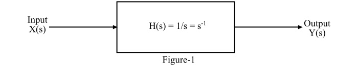
Integrator
- The integrator is an element which is used to integrate the input signal of a system.
- The transfer function of an ideal integrator is given by,
$$\mathrm{H(s)\:=\:\frac{1}{s}\:=\:s^{-1}}$$
- The main advantage of using integrator in the realization of a continuous-time system is that the integrator suppresses the high frequency noise signals. Because of this reason, only integrators are used to realize the practical continuous-time systems.
- The block diagram representation of an ideal integrator is shown in Figure-1.
Adder
- The adder is an element which is used to perform the addition and subtraction of the signals.
- It is also called the summer circuit.
- The output of the adder is the algebraic sum of all the input variables.
- Graphically, it is represented by a small circle that has at least two input terminals and one output terminal as shown in Figure-2.

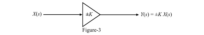
Multiplier
- The multiplier is an element which is used to multiply the input signal by a constant.
- The gain (or constant) of the multiplier can be positive or negative.
- The magnitude of the gain of the multiplier may be greater or less than 1.
- The graphical representation of the multiplier is shown in Figure-3.
When is a continuous-time system not physically realizable?
Consider an nth order continuous-time system represented by the following differential equation −
$$\mathrm{\frac{d^n}{dt^n}\:y(t) \:+\: a_{n-1} \frac{d^{n-1} }{dt^{n-1}}\:y(t) \:+\: a_{n-2} \frac{d^{n-2}}{dt^{n-2}} y(t) \:+\: \dots \:+\: a_1 \frac{d}{dt}y(t) \:+\: a_0 y(t) \:=\: b_m \frac{d^m }{dt^m}x(t) \:+\: b_{m-1} \frac{d^{m-1}}{dt^{m-1}} x(t) \:+\: b_{m-2} \frac{d^{m-2} }{dt^{m-2}}x(t) \:+\: \dots \:+\: b_1 \frac{d}{dt} x(t) \:+\: b_0 x(t)}$$
Taking Laplace transform, we get,
$$\mathrm{s^n \:+\: a_{n-1} s^{n-1} \:+\: a_{n-2} s^{n-2} \:+\: \dots \:+\: a_1 s \:+\: a_0 \:=\: b_m s^m \:+\: b_{m-1} s^{m-1} \:+\: b_{m-2} s^{m-2} \:+\: \dots \:+\: b_1 s \:+\: b_0}$$
Therefore, the transfer function of the system is,
$$\mathrm{H(s) \:=\: \frac{Y(s)}{X(s)} \:=\: \frac{b_m s^m \:+\: b_{m-1} s^{m-1} \:+\: b_{m-2} s^{m-2} \:+\:\dots \:+ \:b_1 s \:+\: b_0}{s^n \:+\: a_{n-1} s^{n-1} \:+\: a_{n-2} s^{n-2} \:+\: \dots \:+\: a_1 s \:+\: a_0}}$$
When m > n, i.e., the order of the numerator polynomial in the transfer function is greater than the order of the denominator polynomial, then the given system is a non-causal system and hence, it is not physically realisable.