- Data Modeling with DAX Tutorial
- Home
- Data Modeling with DAX - Overview
- Data Modeling with DAX - Concepts
- Data Modeling Using Excel Power Pivot
- Loading Data into the Data Model
- Defining Data Types in the Data Model
- Understanding Data Tables
- Extending the Data Model
- Base Finance Measures & Analysis
- YoY Finance Measures & Analysis
- Variance Measures & Analysis
- Year-to-Date Measures & Analysis
- Quarter-to-Date Measures & Analysis
- Budget Measures & Analysis
- Forecast Measures & Analysis
- Count of Months Measures
- Ending Headcount Measures
- Average Headcount Measures
- Total Headcount Measures
- YoY Headcount Measures & Analysis
- Variance Headcount Measures
- Cost Per Headcount Measures & Analysis
- Rate Variance & Volume Variance
- Data Modeling with DAX Resources
- Quick Guide
- Useful Resources
- Discussion
Data Modeling with DAX - Quick Guide
Data Modeling with DAX - Overview
The decision makers in all the organizations have identified the need for analyzing the historical data of their organization in specific, and of the industry in general. This is becoming crucial day-by-day in the present competitive world, to meet the ever-changing business challenges.
Big Data and Business Intelligence have become the buzzwords in the business world. Data sources have become huge and data formats have become variant. The need of the hour is to have simple-to-use tools to handle the ever-flowing vast data in less time to gain insight and make relevant decisions at the appropriate time.
Data analysts can no longer wait for the required data to be processed by the IT department. They require a handy tool that enables them to quickly comprehend the required data and make it available in a format that helps the decision makers take required action at the right time.
Microsoft Excel has a powerful tool called as Power Pivot that was available as an add-in in the prior versions of Excel and is built-in feature in Excel 2016. The database of Power Pivot, called the data model and the formula language that works on the data model, called DAX (Data Analysis Expressions) enables an Excel user to perform tasks such as data modeling and analysis in no time.
In this tutorial, you will learn data modeling and analysis using DAX, based on the Power Pivot data model. A sample Profit and Analysis database is used for the illustrations throughout this tutorial.
Data Modeling and Analysis Concepts
The data that you obtain from different variety of sources, termed as raw data, needs processing before you can utilize it for analysis purposes. You will learn about these in the chapter − Data Modeling and Analysis Concepts.
Data Modeling and Analysis with Excel Power Pivot
Since the tool that you will be mastering in this tutorial is Excel Power Pivot, you need to know how the data modeling and analysis steps are carried out in Power Pivot. You will learn these at a broader level in the chapter - Data Modeling and Analysis with Excel Power Pivot.
As you proceed with the subsequent chapters, you will learn about the different facets of Power Pivot, DAX and DAX functions in data modeling and analysis.
By the end of the tutorial, you will be able to perform data modeling and analysis with DAX for any context at hand.
Data Modeling with DAX - Concepts
Business Intelligence (BI) is gaining importance in several fields and organizations. Decision making and forecasting based on historical data have become crucial in the evergrowing competitive world. There is huge amount of data available both internally and externally from diversified sources for any type of data analysis.
However, the challenge is to extract the relevant data from the available big data as per the current requirements, and to store it in a way that is amicable for projecting different insights from the data. A data model thus obtained with the usage of key business terms is a valuable communication tool. The data model also needs to provide a quick way of generating reports on an as needed basis.
Data modeling for BI systems enables you to meet many of the data challenges.
Prerequisites for a Data Model for BI
A data model for BI should meet the requirements of the business for which data analysis is being done. Following are the minimum basics that any data model has to meet −
The data model needs to be Business Specific
A data model that is suitable for one line of business might not be suitable for a different line of business. Hence, the data model must be developed based on the specific business, the business terms used, the data types, and their relationships. It should be based on the objectives and the type of decisions made in the organization.
The data model needs to have built-in Intelligence
The data model should include built-in intelligence through metadata, hierarchies, and inheritances that facilitate efficient and effective Business Intelligence process. With this, you will be able to provide a common platform for different users, eliminating repetition of the process.
The data model needs to be Robust
The data model should precisely present the data specific to the business. It should enable effective disk and memory storage so as to facilitate quick processing and reporting.
The data model needs to be Scalable
The data model should be able to accommodate the changing business scenarios in a quick and efficient way. New data or new data types might have to be included. Data refreshes might have to be handled effectively.
Data Modeling for BI
Data modeling for BI consists of the following steps −
- Shaping the data
- Loading the data
- Defining the relationships between the tables
- Defining data types
- Creating new data insights
Shaping the Data
The data required to build a data model can be from various sources and can be in different formats. You need to determine which portion of the data from each of these data sources is required for specific data analysis. This is called Shaping the Data.
For example, if you are retrieving the data of all the employees in an organization, you need to decide what details of each employee are relevant to the current context. In other words, you need to determine which columns of the employee table are required to be imported. This is because, the lesser the number of columns in a table in the data model, the faster will be the calculations on the table.
Loading the Data
You need to load the identified data – the data tables with the chosen columns in each of the tables.
Defining the Relationships Between Tables
Next, you need to define the logical relationships between the various tables that facilitate combining data from those tables, i.e. if you have a table – Products - containing data about the products and a table - Sales - with the various sales transactions of the products, by defining a relationship between the two tables, you can summarize the sales, product wise.
Defining Data Types
Identifying the appropriate data types for the data in the data model is crucial for the accuracy of calculations. For each column in each table that you have imported, you need to define the data type. For example, text data type, real number data type, integer data type, etc.
Creating New Data Insights
This is a crucial step in date modeling for BI. The data model that is built might have to be shared with several people who need to understand data trends and make the required decisions in a very short time. Hence, creating new data insights from the source data will be effective, avoiding rework on the analysis.
The new data insights can be in the form of metadata that can be easily understood and used by specific business people.
Data Analysis
Once the data model is ready, the data can be analyzed as per the requirement. Presenting the analysis results is also an important step because the decisions will be made based on the reports.
Data Modeling Using Excel Power Pivot
Microsoft Excel Power Pivot is an excellent tool for data modeling and analysis.
Data model is the Power Pivot database.
DAX is the formula language that can be used to create metadata with the data in the data model by means of DAX formulas.
Power PivotTables in Excel created with the data and metadata in the data model enables you to analyze the data and present the results.
In this tutorial, you will learn data modeling with Power Pivot data model and DAX and data analysis with Power Pivot. If you are new to Power Pivot, please refer to the Excel Power Pivot tutorial.
You have learnt the data modeling process steps in the previous chapter - Data Modeling and Analysis Concepts. In this chapter, you will learn how to execute each of those steps with Power Pivot data model and DAX.
In the following sections, you will learn each of these process steps as applied to Power Pivot data model and how DAX is used.
Shaping the Data
In Excel Power Pivot, you can import data from various types of data sources and while importing, you can view and choose the tables and columns that you want to import.
Identify the data sources.
Find the data source types. For example, database or data service or any other data source.
Decide on what data is relevant in the current context.
Decide on the appropriate data types for the data. In Power Pivot data model, you can have only one data type for the entire column in a table.
Identify which of the tables are the fact tables and which are the dimensional tables.
Decide on the relevant logical relationships between the tables.
Loading Data into the Data Model
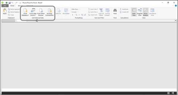
You can load data into the data model with several options provided in the Power Pivot window on the Ribbon. You can find these options in the group, Get External Data.
You will learn how to load data from an Access database into the data model in the chapter – Loading Data into the Data Model.
For illustration purposes, an Access database with Profit and Loss data is used.
Defining Data Types in the Data Model
The next step in the data modeling process in Power Pivot is defining data types of the columns in the tables that are loaded into the data model.
You will learn how to define data types of the columns in the tables in the chapter – Defining Data Types in the Data Model.
Creating Relationships Between the Tables
The next step in the data modeling process in Power Pivot is creating relationships between the tables in the data model.
You will learn how to create relationships between the tables in the chapter – Extending the Data Model.
Creating New Data Insights
In the data model, you can create metadata necessary for creating new data insights by −
- Creating Calculated Columns
- Creating Date Table
- Creating Measures
You can then analyze the data by creating dynamic Power PivotTables that are based on the columns in the tables and measures that appear as fields in the PivotTable Fields list.
Adding Calculated Columns
Calculated columns in a table are the columns that you add to a table by using DAX formulas.
You will learn how to add calculated columns in a table in the data model in the chapter - Extending the Data Model.
Creating Date Table
To use Time Intelligence Functions in DAX formulas to create metadata, you require a Date table. If you are new to Date tables, please refer to the chapter – Understanding Date Tables.
You will learn how to create a Date table in the data model in the chapter – Extending the Data Model.
Creating Measures
You can create various measures in the Data table by using the DAX functions and DAX formulas for different calculations as required for data analysis in the current context.
This is the crucial step of data modeling with DAX.
You will learn how to create the measures for various purposes of profit and loss analysis in the subsequent chapters.
Analyzing Data with Power PivotTables
You can create Power PivotTables for each of the facets of profit and loss analysis. As you learn how to create measures using DAX in the subsequent chapters, you will also learn how to analyze data with these measures using Power PivotTables.
Loading Data into the Data Model
You can load data from different types of data sources into the data model. For this, you can find various options in the Get External Data group on the Ribbon in the Power Pivot window.
As you can observe, you can load data from databases, or from data services or several other types of data sources.
When you load data from a data source into the data model, a connection will be established with the data source. This enables data refresh when the source data changes.
Initiating with a New Data Model
In this section, you will learn how to model the data for profit and loss analysis. The data for analysis is in a Microsoft Access database.
You can initiate a new data model as follows −
- Open a new Excel workbook
- Click the PowerPivot tab on the Ribbon
- Click Manage in the Data Model group
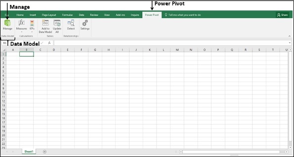
The Power Pivot window appears. The window will be blank as you have not yet loaded any data.
Loading Data from Access Database into the Data Model
To load the data from the Access database, carry out the following steps −
- Click From Database in the Get External Data group on the Ribbon.
- Click From Access in the dropdown list.
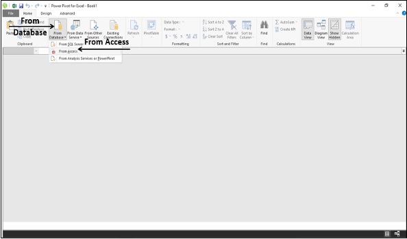
Table Import Wizard dialog box appears.
Browse to the Access file.
Give a friendly name for the connection.
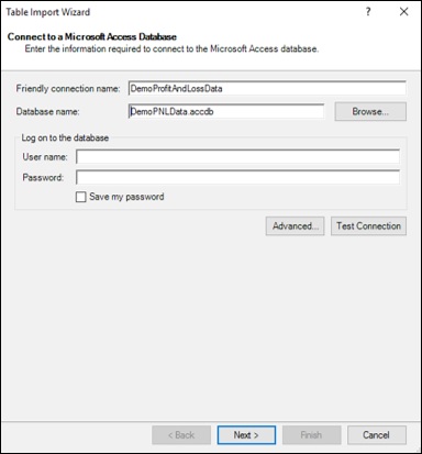
Click the Next button. The next part of the Table Import Wizard appears.
In the Table Import Wizard, select the option – Select from a list of tables and views to choose the data to import.
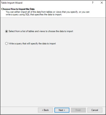
Click the Next button. The next part of the Table Import Wizard appears as shown in the following screenshot.
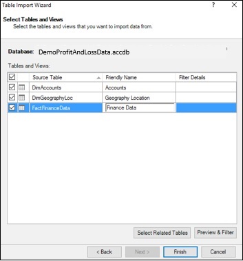
Select all the tables.
Give friendly names to the tables. This is necessary because these names appear in the Power PivotTables and hence should be understood by everyone.
Choosing the Columns in the Tables
You might not require all the columns in the selected tables for the current analysis. Hence, you need to select only those columns that you selected while shaping the data.
Click the Preview & Filter button. The next part of the Table Import Wizard -Preview of the selected table - appears.
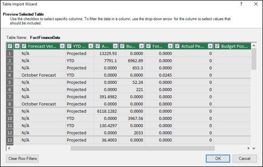
As seen in the above screenshot, the column headers have check boxes. Select the columns you want to import in the selected table.
Click OK. Repeat the same for the other tables.
Importing Data into the Data Model
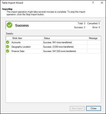
You are at the last stage of loading data into the data model. Click the Finish button in the Table Import Wizard. The next part of the Table Import Wizard appears.
The importing status will be displayed. The status finally displays Success when data loading is complete.
Viewing the Data in the Data Model
The imported tables appear in the Power Pivot window. This is the view of the data model
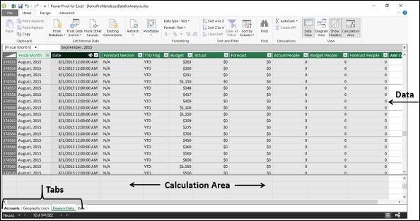
You can observe the following −
- Each of the tables appear in a separate tab.
- The tab names are the respective table names.
- The area below the data is for the calculations.
Viewing the Connection Name
Click the Existing Connections in the Get External Data group. Existing Connections dialog box appears as shown in the following screenshot.
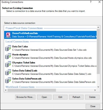
As seen in the above screenshot, the connection name given appears under PowerPivot Data Connections.
Defining Data Types in the Data Model
In the Power Pivot data model, the entire data in a column must be of the same data type. To accomplish accurate calculations, you need to ensure that the data type of each column in each table in the data model is as per requirement.
Tables in the Data Model
In the data model created in the previous chapter, there are 3 tables −
- Accounts
- Geography Locn
- Finance Data
Ensuring Appropriate Data Types
To ensure that the columns in the tables are as required, you need to check their data types in the Power Pivot window.
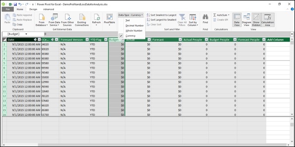
Click a column in a table.
Note the data type of the column as displayed on the Ribbon in the Formatting group.
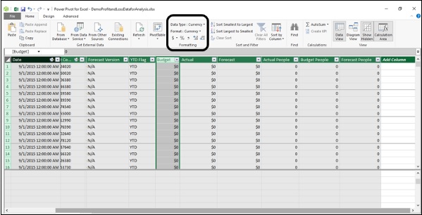
If the data type of the selected column is not appropriate, change the data type as follows.
Click the down arrow next to the data type in the Formatting group.
Click the appropriate data type in the dropdown list.
Repeat for every column in all the tables in the data model.
Columns in the Accounts Table
In the Accounts table, you have the following columns −
| Sr.No | Column & Description |
|---|---|
| 1 | Account
Contains one account number for each row. The column has unique values and is used in defining the relationship with the Finance Data table. |
| 2 | Class
The class associated with each account. Example - Expenses, Net Revenue, etc. |
| 3 | Sub Class
Describes the type of expense or revenue. Example – People. |
All the columns in the Accounts table are of descriptive in nature and hence are of Text data type.
Columns in the Geography Locn Table
The Geography Locn table contains data about each Profit Center.
The column Profit Center contains one profit center identity for each row. This column has unique values and is used in defining the relationship with the Finance Data table.
Columns in the Finance Data Table
In the Finance Data table, you have the following columns −
| Column | Description | Data type |
|---|---|---|
| Fiscal Month | Month and Year | Text |
| Profit Center | Profit Center identity | Text |
| Account | Account number. Each account can have multiple Profit Centers. |
Text |
| Budget | Monthly budget amounts for each Profit Center. | Currency |
| Actual | Monthly actual amounts for each Profit Center. | Currency |
| Forecast | Monthly forecast amounts for each profit center. | Currency |
| Actual People | Month end actual number of employees for each Profit Center of each people Account. | Whole Number |
| Budget People | Month end budget number of employees for each Profit Center of each people Account. | Whole Number |
| Forecast People | Month end forecast number of employees for each Profit Center of each people Account. | Whole Number |
Types of Tables in the Data Model
Both Accounts and Geography Locn tables are the dimensional tables, also called as lookup tables.
Finance Data table is the fact table, also known as the data table. Finance Data table contains the data required for the profit and analysis calculations. You will also create metadata in the form of measures and calculated columns in this Finance Data table, so as to model the data for various types of profit and loss calculations, as you proceed with this tutorial.
Understanding Data Tables
Data Analysis involves browsing data over time and making calculations across time periods. For example, you might have to compare the current year’s profits with the previous year’s profits. Similarly, you might have to forecast the growth and profits in the coming years. For these, you need to use grouping and aggregations over a period of time.
DAX provides several Time Intelligence functions that help you perform most of such calculations. However, these DAX functions require a Date table for usage with the other tables in the data model.
You can either import a Date table along with other data from a data source or you can create a Date table by yourself in the data model.
In this chapter, you will understand different aspects of Date tables. If you are conversant with Date tables in the Power Pivot data model, you can skip this chapter and proceed with the subsequent chapters. Otherwise, you can understand the Date tables in the Power Pivot data model.
What is a Date Table?
A Date Table is a table in a data model, with at least one column of contiguous dates across a required duration. It can have additional columns representing different time periods. However, what is necessary is the column of contiguous dates, as required by the DAX Time Intelligence functions.
For example,
A Date table can have columns such as Date, Fiscal Month, Fiscal Quarter, and Fiscal Year.
A Date table can have columns such as Date, Month, Quarter, and Year.
Date Table with Contiguous Dates
Suppose you are required to make calculations in the range of a calendar year. Then, the Date table must have at least one column with a contiguous set of dates, including all the dates in that specific calendar year.
For example, suppose the data you want to browse has dates from April 1st, 2014 through November 30th, 2016.
If you have to report on a calendar year, you need a Date table with a column – Date, which contains all the dates from January 1st, 2014 to December 31st, 2016 in a sequence.
If you have to report on a fiscal year, and your fiscal year end is 30th June, you need a Date table with a column – Date, which contains all the dates from July 1st, 2013 to June 30th, 2017 in a sequence.
If you have to report on both calendar and fiscal years, then you can have a single Date table spanning the required range of dates.
Your Date table must contain all of the days for the range of every year in the given duration. Thus, you will get contiguous dates within that period of time.
If you regularly refresh your data with new data, you will have the end date extended by a year or two, so that you do not have to update your Date table often.
A Date table looks like the following screenshot.
Adding a Date Table to the Data Model
You can add a Date table to the data model in any of the following ways −
Importing from a relational database, or any other data source.
Creating a Date table in Excel and then copying or linking to a new table in Power Pivot.
Importing from Microsoft Azure Marketplace.
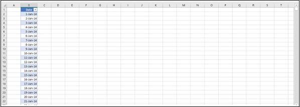
Creating a Date Table in Excel and Copying to the Data Model
Creating a Date table in Excel and copying to the data model is the easiest and most flexible way of creating a Data table in the data model.
Open a new worksheet in Excel.
Type – Date in the first row of a column.
Type the first date in the date range that you want to create in the second row in the same column.
Select the cell, click the fill handle and drag it down to create a column of contiguous dates in the required date range.
For example, type 1/1/2014, click the fill handle and drag down to fill the contiguous dates up to 31/12/2016.
- Click the Date column.
- Click the INSERT tab on the Ribbon.
- Click Table.
- Verify the table range.
- Click OK.
The table of a single column of dates is ready in Excel.
- Select the table.
- Click Copy on the Ribbon.
- Click the Power Pivot window.
- Click Paste on the Ribbon.
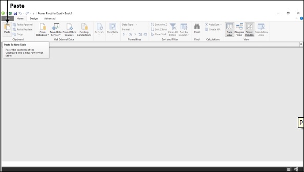
This will add the contents of the clipboard to a new table in the data model. Hence, you can use the same method to create a Date table in an existing data model also.
Paste preview dialog box appears as shown in the following screenshot.
- Type Date in the Table Name box.
- Preview the data.
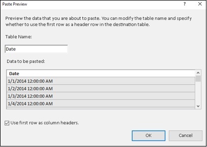
- Check the box – Use first row as column headers.
- Click OK.
This copies the contents of the clipboard to a new table in the data model.
Now, you have a Date table in the data model with a single column of contiguous dates. The header of the column is Date as you had given in the Excel table.
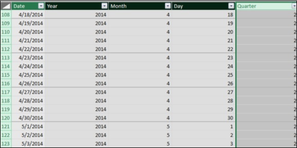
Adding New Date Columns to the Date Table
Next, you can add calculated columns to the Date table as per the requirement for your calculations.
For example, you can add columns – Day, Month, Year, and Quarter as follows −
- Day
=DAY('Date'[Date])
- Month
=MONTH('Date'[Date])
- Year
=YEAR('Date'[Date])
- Quarter
=CONCATENATE ("QTR ", INT (('Date'[Month]+2)/3))
The resulting Date table in the data model looks like the following screenshot.
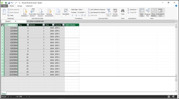
Thus, you can add any number of calculated columns to the Date table. What is important and is required is that the Date table must have a column of contiguous dates that spans the duration of time over which you perform calculations.
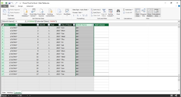
Creating a Date Table for a Calendar Year
A calendar year typically includes the dates from 1st January to 31st December of a year and also includes the holidays marked for that particular year. When you perform calculations, you might have to take into account only the working days, excluding weekends and holidays.
Suppose, you want to create a Date table for the calendar year 2017.
Create an Excel table with a column Date, consisting of contiguous dates from 1st January 2017 to 31st December 2017. (Refer to the previous section to know how to do this.)
Copy the Excel table and paste it into a new table in the data model. (Refer to the previous section to know how to do this.)
Name the table as Calendar.
Add the following calculated columns −
Day =DAY('Calendar'[Date])
Month =MONTH('Calendar'[Date])
Year =YEAR('Calendar'[Date])
Day of Week =FORMAT('Calendar'[Date],"DDD")
Month Name =FORMAT('Calendar'[Date],"MMM")
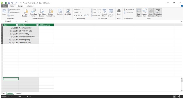
Adding Holidays to the Calendar Table
Add holidays to the Calendar Table as follows −
Get the list of declared holidays for the year.
For example, for the US, you can get the list of holidays for any required year from the following link http://www.calendar-365.com/.
Copy and paste them into an Excel worksheet.
Copy the Excel table and paste it into a new table in the data model.
Name the table as Holidays.
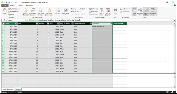
Next, you can add a calculated column of holidays to the Calendar table using DAX LOOKUPVALUE function.
=LOOKUPVALUE(Holidays[Holiday],Holidays[Date],'Calendar'[Date])
DAX LOOKUPVALUE function searches the third parameter, i.e. Calendar[Date] in the second parameter, i.e. Holidays[Date] and returns the first parameter, i.e. Holidays[Holiday] if there is a match. The result will look like what is shown in the following screenshot.
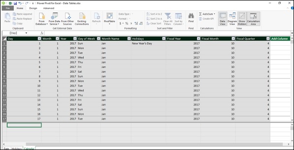
Adding Columns to a Fiscal Year
A fiscal year typically includes the dates from 1st of the month after the fiscal year end to the next fiscal year end. For example, if the fiscal year end is 31st March, then the fiscal year ranges from 1st April to 31st March.
You can include the fiscal time periods in the calendar table using the DAX formulas −
Add a measure for FYE
FYE:=3
Add the following calculated columns −
Fiscal Year
=IF('Calendar'[Month]<='Calendar'[FYE],'Calendar'[Year],'Calendar'[Year]+1)
Fiscal Month
=IF('Calendar'[Month]<='Calendar'[FYE],12-'Calendar'[FYE]+'Calendar'[Month],'Calendar'[Month]-'Calendar'[FYE] )
Fiscal Quarter
=INT(('Calendar'[Fiscal Month]+2)/3)
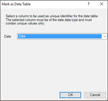
Setting the Date Table Property
When you use DAX Time Intelligence functions such as TOTALYTD, PREVIOUSMONTH, and DATESBETWEEN, they require metadata to work correctly. Date Table Property sets such metadata.
To set the Date Table property −
- Select Calendar table in the Power Pivot window.
- Click the Design tab on the Ribbon.
- Click Mark as Date Table in the Calendars group.
- Click Mark as Date Table in the dropdown list.
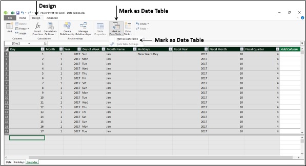
Mark as Date Table dialog box appears. Select the Date column in the Calendar table. This has to be the column of Date data type and has to have unique values. Click OK.
Extending the Data Model
In this chapter, you will learn how to extend the data model created in the previous chapters. Extending a data model includes −
- Addition of tables
- Addition of calculated columns in an existing table
- Creation of measures in an existing table
Of these, creating the measures is crucial, as it involves providing new data insights in the data model that will enable those using the data model avoid rework and also save time while analyzing the data and decision making.
As Profit and Loss Analysis involves working with time periods and you will be using DAX Time Intelligence functions, you require a Date table in the data model.
If you are new to Date tables, go through the chapter – Understanding Date Tables.
You can extend the data model as follows −
To create a relationship between the data table, i.e. Finance Data table and the Date table, you need to create a calculated column Date in the Finance Data table.
To perform different types of calculations, you need to create relationships between the data table - Finance Data and the lookup tables – Accounts and Geography Locn.
You need to create various measures that help you perform several calculations and carry out the required analysis.
These steps essentially constitute the data modeling steps for Profit and Loss Analysis using the data model. However, this is the sequence of steps for any type of data analysis that you want to perform with Power Pivot data model.
Further, you will learn how to create the measures and how to use them in the Power PivotTables in the subsequent chapters. This will give you sufficient understanding of data modeling with DAX and data analysis with Power PivotTables.
Adding a Date Table to the Data Model
Create a Date table for the time periods spanning the fiscal years as follows −
Create a table with a single column with header – Date and contiguous dates ranging from 7/1/2011 to 6/30/2018 in a new Excel worksheet.
Copy the table from Excel and paste it into the Power Pivot window. This will create a new table in the Power Pivot data model.
Name the table as Date.
Ensure that the Date column in the Date table is of data type - Date (DateTime).
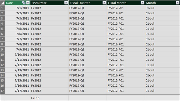
Next, you need to add the calculated columns – Fiscal Year, Fiscal Quarter, Fiscal Month and Month to the Date table as follows −
Fiscal Year
Suppose the fiscal year end is June 30th. Then, a fiscal year spans from 1st July to 30th June. For example, the period July 1st, 2011 (7/1/2011) to June 30th, 2012 (6/30/2012) will be the fiscal year 2012.
In the Date table, suppose you want to represent the same as FY2012.
You need to first extract the financial year part of the Date and append it with FY.
For the dates in the months July 2011 to December 2011, the financial year is 1+2011.
For the dates in the months January 2012 to June 2012, the financial year is 0+2012.
To generalize, if the Month of Financial Year End is FYE, do the following −
Integer Part of ((Month – 1)/FYE) + Year
Next, take the rightmost 4 characters to obtain the Financial Year.
In DAX, you can represent the same as −
RIGHT(INT((MONTH('Date'[Date])-1)/'Date'[FYE])+YEAR('Date'[Date]),4)
Add the calculated column Fiscal Year in the Date table with the DAX formula −
="FY"&RIGHT(INT((MONTH('Date'[Date])-1)/'Date'[FYE])+YEAR('Date'[Date]),4)
Fiscal Quarter
If FYE represents the month of financial year end, the financial quarter is obtained as
Integer Part of ((Remainder of ((Month+FYE-1)/12) + 3)/3)
In DAX, you can represent the same as −
INT((MOD(MONTH('Date'[Date])+'Date'[FYE]-1,12)+3)/3)
Add the calculated column Fiscal Quarter in the Date table with the DAX formula −
='Date'[FiscalYear]&"-Q"&FORMAT( INT((MOD(MONTH('Date'[Date]) + 'Date'[FYE]-1,12) + 3)/3), "0")
Fiscal Month
If FYE represents the financial year end, the financial month period is obtained as
(Remainder of (Month+FYE-1)/12) + 1
In DAX, you can represent the same as −
MOD(MONTH('Date'[Date])+'Date'[FYE]-1,12)+1
Add the calculated column Fiscal Month in the Date table with the DAX formula −
='Date'[Fiscal Year]&"-P" & FORMAT(MOD(MONTH([Date])+[FYE]-1,12)+1,"00")
Month
Finally, add the calculated column Month that represents the month number in a financial year as follows −
=FORMAT(MOD(MONTH([Date])+[FYE]-1,12)+1,"00") & "-" & FORMAT([Date],"mmm")
The resulting Date table looks like the following screenshot.
Mark the table – Date as Date Table with the column - Date as the column with unique values as shown in the following screenshot.
Adding Calculated Columns
To create a relationship between the Finance Data table and the Date table, you require a column of Date values in the Finance Data table.
Add a calculated column Date in the Finance Data table with the DAX formula −
= DATEVALUE ('Finance Data'[Fiscal Month])
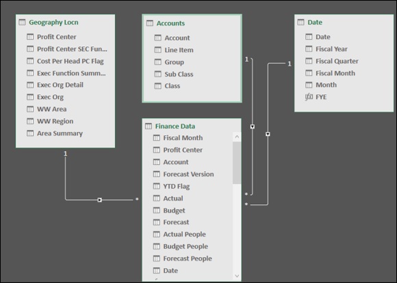
Defining Relationships Between Tables in the Data Model
You have the following tables in the data model −
- Data table - Finance Data
- Lookup tables - Accounts and Geography Locn
- Date table - Date
To define Relationships between the tables in the data model, following are the steps −
View the tables in the Diagram View of the Power Pivot.
Create the following relationships between the tables −
Relationship between Finance Data table and Accounts table with the column Account.
Relationship between Finance Data table and Geography Locn table with the column Profit Center.
Relationship between Finance Data table and Date table with the column Date.
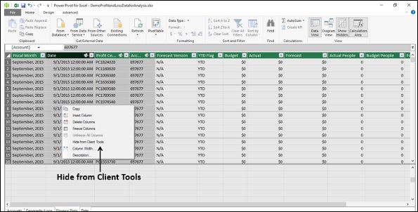
Hiding Columns from Client Tools
If there are any columns in a data table that you won’t be using as fields in any PivotTable, you can hide them in the data model. Then, they will not be visible in the PivotTable Fields list.
In the Finance Data table, you have 4 columns – Fiscal Month, Date, Account and Profit Center that you won’t be using as fields in any PivotTable. Hence, you can hide them so that they do not appear in the PivotTable Fields list.
Select the columns - Fiscal Month, Date, Account, and Profit Center in the Finance Data table.
Right-click and select Hide from Client Tools in the dropdown list.
Creating Measures in the Tables
You are all set for data modeling and analysis with DAX using the data model and Power PivotTables.
In the subsequent chapters, you will learn how to create measures and how to use them in Power PivotTables. You will create all the measures in the data table, i.e. Finance Data table.
You will create measures using DAX formulas in the data table – Finance Data, which you can use in any number of PivotTables for the data analysis. The measures are essentially the metadata. Creating measures in the data table is part of data modeling and summarizing them in the Power PivotTables is part of data analysis.
Base Finance Measures and Analysis
You can create various measures in the data model to be used in any number of Power PivotTables. This forms the data modeling and analysis process with the data model using DAX.
As you have learnt earlier in the previous sections, data modeling and analysis is dependent on specific business and context. In this chapter, you will learn data modeling and analysis based on a sample Profit and Loss database to understand how to create the required measures and use them in various Power PivotTables.
You can apply the same method for data modeling and analysis for any business and context
Creating Measures Based on Finance Data
To create any financial report, you need to make calculations of amounts for a particular time period, organization, account, or geographical location. You also need to perform the headcount and cost per headcount calculations. In the data model, you can create base measures that can be reused in creating other measures. This is an effective way of data modeling with DAX.
In order to perform calculations for profit and loss data analysis, you can create measures such as sum, year-over-year, year-to-date, quarter-to-date, variance, headcount, cost per headcount, etc. You can use these measures in the Power PivotTables to analyze the data and report the analysis results.
In the following sections, you will learn how to create the base finance measures and analyze data with those measures. The measures are termed as base measures as they can be used in creating other financial measures. You will also learn how to create measures for the previous time periods and use them in the analysis.
Creating Base Finance Measures
In the finance data analysis, budget and forecast play a major role.
Budget
A budget is an estimate of a company’s revenues and expenses for a financial year. The budget is calculated at the beginning of a financial year keeping in view the company’s goals and targets. Budget measures need to be analyzed from time to time during the financial year, as the market conditions may change and the company may have to align its goals and targets to the current trends in the industry.
Forecast
A financial forecast is an estimate of a company's future financial outcomes by examining the company’s historical data of revenues and expenses. You can use financial forecasting for the following −
To determine how to allocate budget for a future period.
To track the expected performance of the company.
To take timely decisions to address shortfalls against the targets, or to maximize an emerging opportunity.
Actuals
To perform the budgeting and forecasting calculations, you require the actual revenue and expenses at any point in time.
You can create the following 3 base finance measures that can be used in creating other financial measures in the data mode −
- Budget Sum
- Actual Sum
- Forecast Sum
These measures are the aggregation sums over the columns – Budget, Actual, and Forecast in the Finance Data table.
Create the base finance measures as follows −
Budget Sum
Budget Sum:=SUM('Finance Data'[Budget])
Actual Sum
Actual Sum:=SUM('Finance Data'[Actual])
Forecast Sum
Forecast Sum:=SUM('Finance Data'[Forecast])
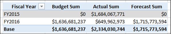
Analyzing Data with Base Finance Measures
With the base finance measures and the Date table, you can perform your analysis as follow −
- Create a Power PivotTable.
- Add the field Fiscal Year from the Date table to Rows.
- Add the measures Budget Sum, Actual Sum, and Forecast Sum (that appear as fields in the PivotTable Fields list) to Values.
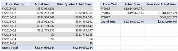
Creating Finance Measures for Previous Periods
With the three base finance measures and the Date table, you can create other finance measures.
Suppose you want to compare the Actual Sum of a Quarter with the Actual Sum of previous Quarter. You can create the measure - Prior Quarter Actual Sum.
Prior Quarter Actual Sum:=CALCULATE([Actual Sum], DATEADD('Date'[Date],1,QUARTER))
Similarly, you can create the measure - Prior Year Actual Sum.
Prior Year Actual Sum:=CALCULATE([Actual Sum], DATEADD('Date'[Date],1,YEAR))
Analyzing Data with Finance Measures for Previous Periods
With the base measures, measures for previous periods and the Date table, you can perform your analysis as follows −
- Create a Power PivotTable.
- Add the field Fiscal Quarter from the Date table to Rows.
- Add the measures Actual Sum and Prior Quarter Actual Sum to Values.
- Create another Power PivotTable.
- Add the field Fiscal Year from the Date table to Rows.
- Add the measures Actual Sum and Prior Year Actual Sum to Values.
YoY Finance Measures and Analysis
Year-over-Year (YoY) is a measure of growth. It is obtained by subtracting the actual sum of the previous year from the actual sum.
If the result is positive, it reflects an increase in actual, and if it is negative, it reflects a decrease in actual, i.e. if we calculate year-over-year as −
year-over-year = (actual sum –prior year actual sum)
- If the actual sum > the prior year actual sum, year-over-year will be positive.
- If the actual sum < the prior year actual sum, year-over-year will be negative.
In the financial data, accounts such as the expense accounts will have debit (positive) amounts and the revenue accounts will have credit (negative) amounts. Hence, for the expense accounts, the above formula works fine.
However, for the revenue accounts, it should be the reverse, i.e.
- If the actual sum > the prior year actual sum, year-over-year should be negative.
- If the actual sum < the prior year actual sum, year-over-year should be positive.
Hence for the revenue accounts, you have to calculate year-over-year as −
year-over-year = -(actual sum – prior year actual sum)
Creating Year-over-Year Measure
You can create Year-over-Year measure with the following DAX formula −
YoY:=IF(CONTAINS(Accounts, Accounts[Class],"Net Revenue"),-([Actual Sum]-[Prior Year Actual Sum]), [Actual Sum]-[Prior Year Actual Sum])
In the above DAX formula −
DAX CONTAINS function returns TRUE, if a row has "Net Revenue" in the column Class in the Accounts table.
DAX IF function then returns –([Actual Sum]-[ Prior Year Actual Sum]).
Otherwise, DAX IF function returns [Actual Sum]-[ Prior Year Actual Sum].
Creating Year-over-Year Percentage Measure
You can represent Year-over-Year as a percentage with the ratio −
(YoY) / (Prior Year Actual Sum)
You can create the Year-over-Year Percentage measure with the following DAX formula −
YoY %:=IF([Prior Year Actual Sum], [YoY] / ABS([Prior Year Actual Sum]),BLANK())
DAX IF function is used in the above formula to ensure that there is no division by zero.
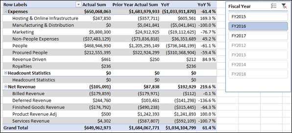
Analyzing Data with Year-over-Year Measures
Create a Power PivotTable as follows −
- Add the fields Class and Sub Class from the Accounts table to Rows.
- Add the measures – Actual Sum, Prior Year Actual Sum, YoY and YoY % to Values.
- Insert a Slicer on the field Fiscal Year from the Date table.
- Select FY2016 in the Slicer.
Creating Budget Year-over-Year Measure
You can create Budget Year-over-Year measure as follows −
Budget YoY: = IF(CONTAINS(Accounts,Accounts[Class],"Net Revenue"), - ([Budget Sum] - [Prior Year Actual Sum]), [Budget Sum] - [Prior Year Actual Sum])
Creating Budget Year-over-Year Percentage Measure
You can create Budget Year-over-Year Percentage measure as follows −
Budget YoY %:=IF([Prior Year Actual Sum] , [Budget YoY] / ABS ([Prior Year Actual Sum]) , BLANK())
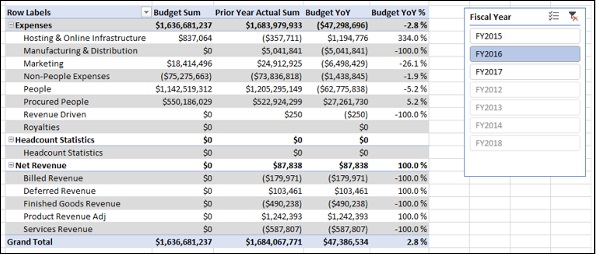
Analyzing Data with Budget Year-over-Year Measures
Create a Power PivotTable as follows −
- Add the fields Class and Sub Class from the Accounts table to Rows.
- Add the measures – Budget Sum, Prior Year Actual Sum, Budget YoY and Budget YoY % to Values.
- Insert a Slicer on the field Fiscal Year from the Date table.
- Select FY2016 in the Slicer.
Creating Forecast Year-over-Year Measure
You can create Forecast Year-over-Year measure as follows −
Forecast YoY:=IF(CONTAINS(Accounts,Accounts[Class],"Net Revenue"), - ([Forecast Sum] - [Prior Year Actual Sum]), [Forecast Sum] - [Prior Year Actual Sum])
Creating Forecast Year-over-Year Percentage Measure
You can create Forecast Year-over-Year Percentage measure as follows −
Forecast YoY %:=IF([Prior Year Actual Sum],[Forecast YoY]/ABS([Prior Year Actual Sum]),BLANK())
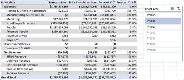
Analyzing Data with Forecast Year-over-Year Measures
Create a Power PivotTable as follows −
- Add the fields Class and Sub Class from the Accounts table to Rows.
- Add the measures – Forecast Sum, Prior Year Actual Sum, Forecast YoY and Forecast YoY % to Values.
- Insert a Slicer on the field Fiscal Year from the Data table.
- Select FY2016 in the Slicer.
Variance Measures and Analysis
You can create variance measures such as variance to budget, variance to forecast, and forecast variance to budget. You can also analyze the finance data based on these measures.
Creating Variance to Budget Sum Measure
Create Variance to Budget Sum measure (VTB Sum) as follows −
VTB Sum:=[Budget Sum]-[Actual Sum]
Creating Variance to Budget Percentage Measure
Create Variance to Budget Percentage measure (VTB %) as follows −
VTB %:=IF([Budget Sum],[VTB Sum]/ABS([Budget Sum]),BLANK())
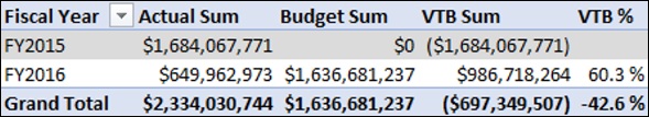
Analyzing Data with Variance to Budget Measures
Create a Power PivotTable as follows −
- Add Fiscal Year from the Date table to Rows.
- Add the measures Actual Sum, Budget Sum, VTB Sum, VTB % from the Finance Data table to Values.
Creating Variance to Forecast Sum Measure
Create Variance to Forecast Sum (VTF Sum) measure as follows −
VTF Sum:=[Forecast Sum]-[Actual Sum]
Creating Variance to Forecast Percentage Measure
Create Variance to Forecast Percentage measure (VTF %) as follows −
VTF %:=IF([Forecast Sum],[VTF Sum]/ABS([Forecast Sum]),BLANK())
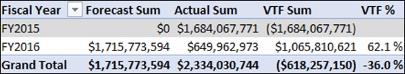
Analyzing Data with Variance to Forecast Measures
Create a Power PivotTable as follows −
- Add Fiscal Year from the Date table to Rows.
- Add the measures Actual Sum, Forecast Sum, VTF Sum, VTF % from the Finance Data table to Values.
Creating Forecast Variance to Budget Sum Measure
Create Forecast Variance to Budget Sum (Forecast VTB Sum) measure as follows −
Forecast VTB Sum:=[Budget Sum]-[Forecast Sum]
Creating Forecast Variance to Budget Percentage Measure
Create Forecast Variance to Budget Percentage (Forecast VTB Percentage) measure as follows −
Forecast VTB %:=IF([Budget Sum],[Forecast VTB Sum]/ABS([Budget Sum]),BLANK())
Analyzing Data with Forecast Variance to Budget Measures
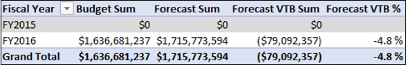
Create a Power PivotTable as follows −
- Add Fiscal Year from the Date table to Rows.
- Add the measures Budget Sum, Forecast Sum, Forecast VTB Sum, Forecast VTB % from the Finance Data table to Values.
Year-to-Date Measures and Analysis
To calculate a result that includes a starting balance from the beginning of a period, such as a fiscal year, up to a specific period in time, you can use DAX Time Intelligence functions. This will enable you to analyze data on a month level.
In this chapter, you will learn how to create Year-to-Date measures and how to carry out data analysis with the same.
Creating Year-to-Date Actual Sum Measure
Create Year-to-Date Actual Sum measure as follows −
YTD Actual Sum:=TOTALYTD([Actual Sum], 'Date'[Date], ALL('Date'), "6/30")
Creating Year-to-Date Budget Sum Measure
Create Year-to-Date Budget Sum measure as follows −
YTD Budget Sum:=TOTALYTD([Budget Sum], 'Date'[Date], ALL('Date'), "6/30")
Creating Year-to-Date Forecast Sum Measure
Create Year-to-Date Forecast Sum measure as follows −
YTD Forecast Sum:=TOTALYTD([Forecast Sum], 'Date'[Date], ALL('Date'), "6/30")
Creating Prior Year-to-Date Actual Sum Measure
Create Prior Year-to-Date Actual Sum measure as follows −
Prior YTD Actual Sum:=TOTALYTD([Prior Year Actual Sum], 'Date'[Date], ALL('Date'), "6/30")
Analyzing Data with Year-to-Date Measures
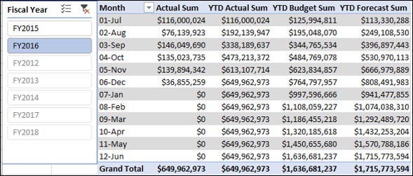
Create a Power PivotTable as follows −
Add Month from Date table to Rows.
Add the measures Actual Sum, YTD Actual Sum, YTD Budget Sum, and YTD Forecast Sum from the Finance Data table to Values.
Insert a Slicer on the Fiscal Year from the Date table.
Select FY2016 in the Slicer.
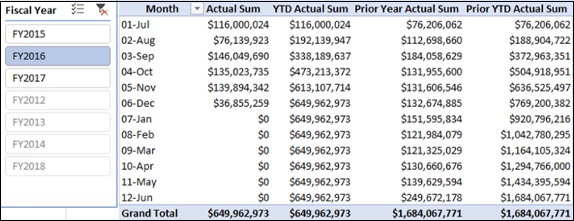
Create a Power PivotTable as follows −
Add Month from Date table to Rows.
Add the measures Actual Sum, YTD Actual Sum, Prior Year Actual Sum, and Prior Year YTD Actual Sum from the Finance Data table to Values.
Insert a Slicer on the Fiscal Year from the Date table.
Select FY2016 in the Slicer.
Quarter-to-Date Measures and Analysis
To calculate a result that includes a starting balance from the beginning of a period, such as a fiscal quarter, up to a specific period in time, you can use DAX Time Intelligence functions. This will enable you to analyze data on a month level.
In this chapter, you will learn how to create Quarter-to-Date measures and how to carry out data analysis with the same.
Creating Quarter-to-Date Sum Measure
Create Quarter-to-Date Actual Sum measure as follows −
QTD Actual Sum:=TOTALQTD([Actual Sum],'Date'[Date],ALL('Date'))
Creating Quarter-to-Date Budget Sum Measure
Create Quarter-to-Date Budget Sum measure as follows −
QTD Budget Sum:=TOTALQTD([Budget Sum], 'Date'[Date], ALL('Date'))
Creating Quarter-to-Date Forecast Sum Measure
Create Quarter-to-Date Budget Sum measure as follows −
QTD Budget Sum:=TOTALQTD([Budget Sum], 'Date'[Date], ALL('Date'))
Creating Quarter-to-Date Forecast Sum Measure
Create Quarter-to-Date Forecast Sum measure as follows −
QTD Forecast Sum:=TOTALQTD([Forecast Sum], 'Date'[Date], ALL('Date'))
Creating Prior Quarter-to-Date Actual Sum Measure
Create Prior Quarter-to-Date Actual Sum measure as follows −
Prior QTD Actual Sum:=TOTALQTD([Prior Quarter Actual Sum], 'Date'[Date], ALL('Date'))
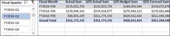
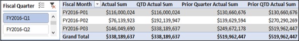
Analyzing Data with Quarter-to-Date Measures
Create a Power PivotTable as follows −
Add Fiscal Month from Date table to Rows.
Add the measures Actual Sum, QTD Actual Sum, QTD Budget Sum, and QTD Forecast Sum from Finance Data table to Values.
Insert a Slicer on the Fiscal Quarter from the Date table.
Select FY2016-Q2 in the Slicer.
Create a Power PivotTable as follows −
Add Fiscal Month from Date table to Rows.
Add the measures Actual Sum, QTD Actual Sum, Prior Quarter Actual Sum, and Prior QTD Actual Sum from Finance Data table to Values.
Insert a Slicer on the Fiscal Quarter from Date table.
Select FY2016-Q1 in the Slicer.
Budget Measures and Analysis
Budgeting involves estimating the cash flows of a company over a financial year. The financial position of the company, its goals, expected revenues, and expenses are taken into account in budgeting.
However, the market conditions may change during the financial year and the company may have to reset its goals. This requires analyzing the financial data with the budget estimated at the beginning of the financial year (Budget Sum) and the actual expended sum from the beginning of the financial year to date (YTD Actual Sum).
At any time during a financial year, you can calculate the following −
Unexpended Balance
Unexpended Balance is the budget remaining after the actual expenses, i.e.
Unexpended Balance = YTD Budget Sum – YTD Actual Sum
Budget Attainment %
Budget Attainment % is the percentage of the budget that you have spent to date, i.e.
Budget Attainment % = YTD Actual Sum/YTD Budget Sum
These calculations help those companies that use budgeting to make decisions.
Creating Unexpended Balance Measure
You can create Unexpended Balance measure as follows −
Unexpended Balance:=CALCULATE( [YTD Budget Sum],ALL('Finance Data'[Date]) )-[YTD Actual Sum]
Creating Budget Attainment Percentage Measure
You can create Budget Attainment Percentage measure as follows −
Budget Attainment %:=IF([YTD Budget Sum],[YTD Actual Sum]/CALCULATE([YTD Budget Sum],ALL('Finance Data'[Date])),BLANK())
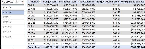
Analyzing Data with Budget Measures
Create a Power PivotTable as follows −
Add Month from the Date table to Rows.
Add the measures Budget Sum, YTD Budget Sum, YTD Actual Sum, Budget Attainment % and Unexpended Balance from Finance Data table to Values.
Insert a Slicer on the Fiscal Year field.
Select FY2016 in the Slicer.
Forecast Measures and Analysis
You can use Forecast measures to analyze the finance data and help an organization make necessary adjustments in its goals and targets for the year, to align the company’s performance to the changing business requirements.
You need to update the forecasts regularly to keep up with the changes. You can then compare the most recent forecast to the budget for the rest of the period in the financial year so that the company can make the required adjustments to meet the business changes.
At any time during a financial year, you can calculate the following −
Forecast Attainment %
Forecast Attainment % is the percentage of the forecast sum that you have spent to date, i.e.
Forecast Attainment % = YTD Actual Sum/YTD Forecast Sum
Forecast Unexpended Balance
Forecast Unexpended Balance is the Forecast Sum remaining after the actual expenses, i.e
Forecast Unexpended Balance = YTD Forecast Sum – YTD Actual Sum
Budget Adjustment
Budget Adjustment is the adjustment in the budget sum an organization needs to make (an increase or decrease) based on the forecast.
Budget Adjustment = Forecast Unexpended Balance - Unexpended Balance
The budget needs to be increased if the resulting value is positive. Otherwise, it can be adjusted for some other purpose.
Creating Forecast Attainment Percentage Measure
You can create Forecast Attainment Percentage measure as follows −
Forecast Attainment Percentage:= IF([YTD Forecast Sum], [YTD Actual Sum]/[YTD Forecast Sum], BLANK())
Creating Forecast Unexpended Balance Measure
You can create Forecast Unexpended Balance measure as follows −
Forecast Unexpended Balance:=[YTD Forecast Sum]-[YTD Actual Sum]
Creating Budget Adjustment Measure
You can create Budget Adjustment measure as follows −
Budget Adjustment:=[Forecast Unexpended Balance]-[Unexpended Balance]
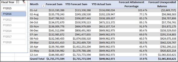
Analyzing Data with Forecast Measures
Create a Power PivotTable as follows −
Add Month from Date table to Rows.
Add the measures Budget Sum, YTD Budget Sum, YTD Actual Sum, Budget Attainment % and Unexpended Balance from Finance Data table to Values.
Insert a Slicer on Fiscal Year.
Select FY2016 in the Slicer.
Count of Months Measures
You can create the Count of Months measures that can be used in creating Headcount measures and Cost Per Head measures. These measures count the distinct values of Fiscal Month column where the Actual column / Budget column / Forecast column has non-zero values in the Finance Data table. This is required because the Finance Data table contains zero values in the Actual column and those rows are to be excluded while calculating Headcount and Cost per Head.
Creating Count of Actual Months Measure
You can create Count of Actual Months measure as follows −
CountOfActualMonths:=CALCULATE(DISTINCTCOUNT('FinanceData' [Fiscal Month]),'Finance Data'[Actual]<>0)
Creating Count of Budget Months Measure
You can create Count of Budget Months measure as follows −
CountOfBudgetMonths:=CALCULATE(DISTINCTCOUNT('FinanceData' [Fiscal Month]),'Finance Data'[Budget]<>0)
Creating Count of Forecast Months Measure
You can create Count of Forecast Months measure as follows −
CountOfForecastMonths:=CALCULATE(DISTINCTCOUNT('FinanceData' [Fiscal Month]),'Finance Data'[Forecast]<>0)
Ending Headcount Measures
You can create Ending Headcount measures for a specific period of time. The Ending Headcount is the sum of the people as on the last date in the specified period for which we have a non-blank sum of people.
The Ending Headcount is obtained as follows −
For a Month − Sum of People at the end of the specific Month.
For a Quarter − Sum of People at the end of the last Month of the specific Quarter.
For a Year − Sum of People at the end of the last Month of the specific Year.
Creating Actual Ending Headcount Measure
You can create Actual Ending Headcount measure as follows −
Actual Ending Head Count:=CALCULATE(SUM('Finance Data'[Actual People]),LASTNONBLANK('Finance Data'[Date], IF(CALCULATE(SUM('Finance Data'[Actual People]), ALL(Accounts))=0, BLANK(), CALCULATE(SUM('Finance Data'[Actual People]), ALL(Accounts)))), ALL(Accounts))
DAX LASTNONBLANK function as used above returns the last date for which you have a non-blank sum of people so that you can calculate the sum of people on that date.
Creating Budget Ending Headcount Measure
You can create Budget Ending Headcount measure as follows −
Budget Ending Head Count: = CALCULATE(SUM('Finance Data'[Budget People]),LASTNONBLANK('Finance Data'[Date], IF(CALCULATE(SUM('Finance Data'[Budget People]), ALL(Accounts))=0, BLANK(), CALCULATE(SUM('Finance Data'[Budget People]), ALL(Accounts)))), ALL(Accounts))
Creating Forecast Ending Headcount Measure
You can create Forecast Ending Headcount measure as follows −
Forecast Ending Head Count:= CALCULATE(SUM('Finance Data'[Forecast People]), LASTNONBLANK('Finance Data'[Date], IF(CALCULATE(SUM('Finance Data'[Forecast People]), ALL(Accounts))=0, BLANK(),CALCULATE(SUM('Finance Data'[Forecast People]), ALL(Accounts)))), ALL(Accounts))
Creating Prior Year Actual Ending Headcount Measuree
You can create Prior Year Actual Ending Headcount measure as follows −
Prior Year Actual Ending Headcount:=CALCULATE('Finance Data'[Actual Ending Head Count], DATEADD('Date'[Date],-1,YEAR))
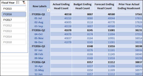
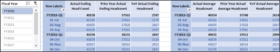
Analyzing Data with Ending Headcount Measures
Create a Power PivotTable as follows −
Add the fields Fiscal Year and Month from the Date table to Rows.
Add the measures Actual Ending Headcount, Budget Ending Headcount, Forecast Ending Headcount, Prior Year Actual Ending Headcount from Finance Data table to Values.
Insert a Slicer on the Fiscal Year field.
Select FY2016 in the Slicer.
Average Headcount Measures
In the previous chapter, you have learnt how to calculate ending headcounts for a specific period. Likewise, you can create the average monthly headcount for any given selection of months.
The Average Monthly Headcount is the sum of the monthly headcounts divided by the number of months in the selection.
You can create these measures using DAX AVERAGEX function.
Creating Actual Average Headcount Measure
You can create Actual Average Headcount measure as follows −
Actual Average Headcount:=AVERAGEX(VALUES('Finance Data'[Fiscal Month]), [Actual Ending Head Count])
Creating Budget Average Headcount Measure
You can create Actual Average Headcount measure as follows −
Budget Average Headcount:=AVERAGEX(VALUES('Finance Data'[Fiscal Month]), [Budget Ending Head Count])
Creating Forecast Average Headcount Measure
You can create Forecast Average Headcount measure as follows −
Forecast Average Headcount:=AVERAGEX( VALUES('Finance Data'[Fiscal Month]), [Actual Ending Head Count])
Creating Prior Year Actual Average Headcount Measure
You can create Prior Year Actual Average Headcount measure as follows −
Prior Year Actual Average Headcount:=CALCULATE('Finance Data'[Actual Average Headcount], DATEADD('Date'[Date], -1, YEAR))
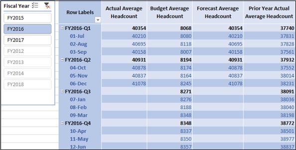
Analyzing Data with Average Headcount Measures
Create a Power PivotTable as follows −
Add the fields Fiscal Year and Month from the Date table to Rows.
Add the measures Actual Average Headcount, Budget Average Headcount, Forecast Average Headcount, Prior Year Actual Average Headcount from Finance Data table to Values.
Insert a Slicer on the Fiscal Year field.
Select FY2016 in the Slicer.
Total Headcount Measures
In the previous chapters, you have learnt how to create Count of Months measures and Average Headcount measures. You can use these measures to calculate the base Headcount Measures −
- Actual Total Headcount
- Budget Total Headcount
- Forecast Total Headcount
In the subsequent chapters, you will learn how to use these base Headcount measures in other calculations such as YoY Headcount and Variance measures.
Creating Actual Total Headcount Measure
You can create Actual Total Headcount Measure as follows −
Actual Total Head Count:= 'Finance Data'[Actual Average Headcount]*'Finance Data'[CountOfActualMonths]
Creating Budget Total Headcount Measure
You can create Budget Total Headcount Measure as follows −
Budget Total Headcount:= 'Finance Data'[Budget Average Headcount]*'Finance Data'[CountOfBudgetMonths]
Creating Forecast Total Headcount Measure
You can create Forecast Total Headcount Measure as follows −
Forecast Total Headcount:= 'Finance Data'[Forecast Average Headcount]*'Finance Data'[CountOfForecastMonths]
YoY Headcount Measures and Analysis
In the previous chapter, you have learnt how to create base Headcount measures – i.e. Actual Total Headcount, Budget Total Headcount, and Forecast Total Headcount.
In this chapter, you will learn how to create Year-Over-Year Headcount measures and how you can analyze the data with these measures.
Creating Year-over-Year Actual Ending Headcount Measure
You can create Year-over-Year Actual Ending Headcount Measure as follows −
YoY Actual Ending Headcount:=[Actual Ending Head Count]-[Prior Year Actual Ending Headcount]
Creating Year-over-Year Actual Average Headcount Measure
You can create Year-over-Year Actual Average Headcount Measure as follows −
YoY Actual Average Headcount:= [Actual Average Headcount]-[Prior Year Actual Average Headcount]
Creating Year-over-Year Actual Total Headcount Measure
You can create Year-over-Year Actual Total Headcount Measure as follows −
YoY Actual Total Headcount:=[Actual Total Head Count]-[Prior Year Actual Total Headcount]
Analyzing Data with Year-over-Year Actual Headcount Measures
Create a Power PivotTable as follows −
Add the fields Fiscal Quarter and Month from the Date table to Rows.
Add the measures – Actual Ending Head Count, Prior Year Actual Ending Head Count, YoY Actual Ending Head Count to Values.
Insert a Slicer on the field Fiscal Year.
Select FY2016 in the Slicer.
Create another Power PivotTable on the same worksheet as follows −
Add the fields Fiscal Quarter and Month from the Date table to Rows.
Add the measures – Actual Average Head Count, Prior Year Actual Average Head Count, YoY Actual Average Head Count to Values.
Connect the Slicer to this PivotTable as follows −
- Click the Slicer.
- Click the Options tab under Slicer Tools on the Ribbon.
- Click Report Connections.
Report Connections dialog box appears.
- Select the above two PivotTables.
- Click OK.
Creating Year-over-Year Budget Ending Headcount Measure
You can create Year-over-Year Budget Ending Headcount Measure as follows −
YoY Budget Ending Headcount:= [Budget Ending Head Count]-[Prior Year Actual Ending Headcount]
Creating Year-over-Year Budget Average Headcount Measure
You can create Year-over-Year Budget Average Headcount Measure as follows −
YoY Budget Average Headcount:= [Budget Average Headcount]-[Prior Year Actual Average Headcount]
Creating Year-over-Year Budget Total Headcount Measure
You can create Year-over-Year Budget Total Headcount Measure as follows −
YoY Budget Total Headcount:=[Budget Total Headcount]-[Prior Year Actual Total Headcount]
Creating Year-over-Year Forecast Ending Headcount Measure
You can create Year-over-Year Forecast Ending Headcount Measure as follows −
YoY Forecast Ending Headcount:= [Forecast Ending Head Count]-[Prior Year Actual Ending Headcount]
Creating Year-over-Year Forecast Average Headcount Measure
You can create Year-over-Year Forecast Average Headcount Measure as follows −
YoY Forecast Average Headcount:= [Forecast Average Headcount]-[Prior Year Actual Average Headcount]
Creating Year-over-Year Forecast Total Headcount Measure
You can create Year-over-Year Forecast Total Headcount Measure as follows −
YoY Forecast Total Headcount:=[Forecast Total Headcount]-[Prior Year Actual Total Headcount]
Variance Headcount Measures
You can create the Variance Headcount measures based on the Headcount measures that you have created so far.
Creating Variance to Budget Ending Headcount Measure
You can create Variance to Budget Ending Headcount Measure as follows −
VTB Ending Head Count:= 'Finance Data'[Budget Ending Head Count]-'Finance Data'[Actual Ending Head Count]
Creating Variance to Budget Average Headcount Measure
You can create Variance to Budget Average Headcount Measure as follows −
VTB Average Head Count:= 'Finance Data'[Budget Average Headcount]-'Finance Data'[Actual Average Headcount
Creating Variance to Budget Total Headcount Measure
You can create Variance to Budget Total Headcount Measure as follows −
VTB Total Head Count:= 'Finance Data'[Budget Total Headcount]-'Finance Data'[Actual Total Head Count]
Creating Variance to Forecast Ending Headcount Measure
You can create Variance to Forecast Ending Headcount Measure as follows −
VTF Ending Head Count:= 'Finance Data'[Forecast Ending Head Count]-'Finance Data'[Actual Ending Head Count]
Creating Variance to Forecast Average Headcount Measure
You can create Variance to Forecast Average Headcount Measure as follows −
VTF Average Head Count:= 'Finance Data'[Forecast Average Headcount]-'Finance Data'[Actual Average Headcount]
Creating Variance to Forecast Total Headcount Measure
You can create Variance to Forecast Total Headcount Measure as follows −
VTF Total Head Count:= 'Finance Data'[Forecast Total Headcount]-'Finance Data'[Actual Total Head Count]
Creating Forecast Variance to Budget Ending Headcount Measure
You can create Forecast Variance to Budget Ending Headcount Measure as follows −
Forecast VTB Ending Head Count:= 'Finance Data'[Budget Ending Head Count]-'Finance Data'[Forecast Ending Head Count]
Creating Forecast Variance to Budget Average Headcount Measure
You can create Forecast Variance to Budget Average Headcount Measure as follows −
Forecast VTB Average Head Count:='Finance Data'[Budget Average Headcount]-'Finance Data'[Forecast Average Headcount]
Creating Forecast Variance to Budget Total Headcount Measure
You can create Forecast Variance to Budget Total Headcount Measure as follows −
Forecast VTB Total Head Count:= 'Finance Data'[Budget Total Headcount]-'Finance Data'[Forecast Total Headcount
Cost Per Headcount Measures and Analysis
You have learnt about the two major categories of Measures −
- Finance Measures.
- Headcount Measures.
The third major category of measures that you will learn is People Cost Measures. Any organization will be interested to know the annualized cost per head. Annualized cost per head represents the cost to the company of having one employee on a full year basis.
To create Cost Per Head measures, you need to first create certain preliminary People Cost Measures. In the Accounts table, you have a column – Sub Class that contains People as one of the values. Hence, you can apply a filter on the Accounts table on the Sub Class column to obtain the filter context onto the Finance Data table to obtain People Cost.
You can use thus obtain People Cost measures and Count of Months measures to create Annualized People Cost measures. You can finally create Annualized Cost Per Head measures from Annualized People Cost measures and Average Head Count measures.
Creating Actual People Cost Measure
You can create Actual People Cost measure as follows −
Actual People Cost:=CALCULATE('Finance Data'[Actual Sum], FILTER('Finance Data', RELATED(Accounts[Sub Class])="People"))
Creating Budget People Cost Measure
You can create Budget People Cost measure as follows −
Budget People Cost:=CALCULATE('Finance Data'[Budget Sum], FILTER('Finance Data', RELATED(Accounts[Sub Class])="People"))
Creating Forecast People Cost Measure
You can create Forecast People Cost measure as follows −
Forecast People Cost:=CALCULATE('Finance Data'[Forecast Sum], FILTER('Finance Data', RELATED(Accounts[Sub Class])="People"))
Creating Annualized Actual People Cost Measure
You can create Annualized Actual People Cost measure as follows −
Annualized Actual People Cost:=IF([CountOfActualMonths],[Actual People Cost]*12/[CountOfActualMonths],BLANK())
Creating Annualized Budget People Cost Measure
You can create Annualized Budget People Cost measure as follows −
Annualized Budget People Cost:=IF([CountOfBudgetMonths], [Budget People Cost]*12/[CountOfBudgetMonths],BLANK())
Creating Annualized Forecast People Cost Measure
You can create Annualized Forecast People Cost measure as follows −
Annualized Forecast People Cost:=IF([CountOfForecastMonths],[Forecast People Cost]*12/[CountOfForecastMonths],BLANK())
Creating Actual Annualized Cost Per Head Measure
You can create Actual Annualized Cost Per Head (CPH) measure as follows −
Actual Annualized CPH:=IF([Actual Average Headcount], [Annualized Actual People Cost]/[Actual Average Headcount],BLANK() )
Creating Budget Annualized Cost Per Head Measure
You can create Budget Annualized Cost Per Head (CPH) measure as follows −
Budget Annualized CPH:=IF([Budget Average Headcount],[Annualized Budget People Cost]/[Budget Average Headcount],BLANK())
Creating Forecast Annualized Cost Per Head Measure
You can create Forecast Annualized Cost Per Head (CPH) measure as follows −
Forecast Annualized CPH:=IF([Forecast Average Headcount],[Annualized Forecast People Cost]/[Forecast Average Headcount], BLANK())
Creating Prior Year Actual Annualized Cost Per Head Measure
You can create Prior Year Actual Annualized Cost Per Head (CPH) measure as follows −
Prior Year Actual Annualized CPH:=CALCULATE([Actual Annualized CPH], DATEADD('Date'[Date],-1,YEAR) )
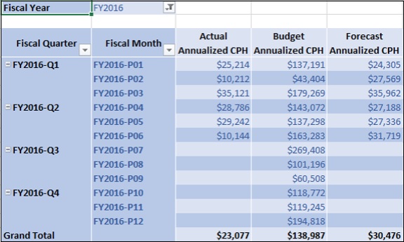
Analyzing Data with Cost Per Head Measures
Create a Power PivotTable as follows −
Add the fields Fiscal Quarter and Fiscal Month from Date table to Rows.
Add the measures Actual Annualized CPH, Budget Annualized CPH, and Forecast Annualized CPH to Columns.
Add the field Fiscal Year from Date table to Filters.
Select FY2016 in the Filter.
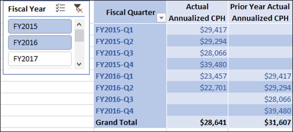
Create another Power PivotTable as follows −
Add the field Fiscal Quarter from Date table to Rows.
Add the measures Actual Annualized CPH, and Prior Year Actual Annualized CPH to Columns.
Insert a Slicer on the field Fiscal Year from Date table.
Select FY2015 and FY2016 on the Slicer.
Rate Variance and Volume Variance
You have learnt how to create measures for Annualized Cost Per Head and Total Headcount. You can use these measures to create Rate Variance and Volume Variance measures.
Rate Variance measures calculate what portion of a Currency Variance is caused by differences in Cost Per Head.
Volume Variance measures calculate how much of the Currency Variance is driven by fluctuation in Headcount.
Creating Variance to Budget Rate Measure
You can create Variance to Budget Rate measure as follows −
VTB Rate:=([Budget Annualized CPH]/12-[Actual Annualized CPH]/12)*[Actual Total Head Count]
Creating Variance to Budget Volume Measure
You can create Variance to Budget Volume measure as follows −
VTB Volume:=[VTB Total Head Count]*[Budget Annualized CPH]/12
Analyzing Data with Variance to Budget Measures
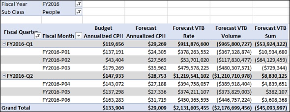
Create a Power PivotTable as follows −
- Add the fields Fiscal Quarter and Fiscal Month from Date table to Rows.
- Add the measures Actual Annualized CPH, Budget Annualized CPH, VTB Rate, VTB Volume, VTB Sum to Values.
- Add the fields Fiscal Year from Date table and Sub Class from Accounts table to Filters.
- Select FY2016 in the Fiscal Year Filter.
- Select People in the Sub Class Filter.
- Filter Row Labels for Fiscal Quarter values FY2016-Q1 and FY2016-Q2.
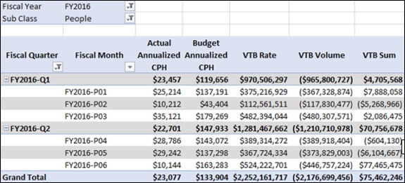
You can observe the following in the above PivotTable −
VTB Sum value shown is only for Sub Class – People.
For Fiscal Quarter FY2016-Q1, VTB Sum is $4,705,568, VTB Rate is $970,506,297, and VTB Volume is $-965,800,727.
VTB Rate measure calculates that $970,506,297 of the Variance to Budget (VTB Sum) is caused by the difference in Cost per Head, and $-965,800,727 is caused by the difference in Headcount.
If you add VTB Rate and VTB Volume, you will get $4,705,568, the same value as returned by VTB Sum for Sub Class People.
Similarly, for Fiscal Quarter FY2016-Q2, VTB Rate is $1,281,467,662, and VTB Volume is $-1,210,710,978. If you add VTB Rate and VTB Volume, you will get $70,756,678, which is the VTB Sum value shown in the PivotTable.
Creating Year-Over-Year Rate Measure
You can create Year-Over-Year Rate measure as follows −
YoY Rate:=([Actual Annualized CPH]/12-[Prior Year Actual Annualized CPH]/12)*[Actual Total Head Count]
Creating Year-Over-Year Volume Measure
You can create Year-Over-Year Volume measure as follows −
YoY Volume:=[YoY Actual Total Headcount]*[Prior Year Actual Annualized CPH]/12
Creating Variance to Forecast Rate Measure
You can create Variance to Forecast Rate measure as follows −
VTF Rate:=([Forecast Annualized CPH]/12-[Actual Annualized CPH]/12)*[Actual Total Head Count]
Creating Variance to Forecast Volume Measure
You can create Variance to Forecast Volume measure as follows −
VTF Volume:=[VTF Total Head Count]*[Forecast Annualized CPH]/12
Analyzing Data with Variance to Forecast Measures
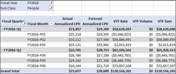
Create a Power PivotTable as follows −
Add the fields Fiscal Quarter and Fiscal Month from Date table to Rows.
Add the measures Actual Annualized CPH, Forecast Annualized CPH, VTF Rate, VTF Volume, VTF Sum to Values.
Add the fields Fiscal Year from Date table and Sub Class from Accounts table to Filters.
Select FY2016 in the Fiscal Year Filter.
Select People in the Sub Class Filter.
Filter Row Labels for Fiscal Quarter values FY2016-Q1 and FY2016-Q2.
Creating Forecast Variance to Budget Rate Measure
You can create Forecast Variance to Budget Rate measure as follows −
Forecast VTB Rate:=([Budget Annualized CPH]/12-[Forecast Annualized CPH]/12)*[Forecast Total Headcount]
Creating Forecast Variance to Budget Volume Measure
You can create Forecast Variance to Budget Volume measure as follows −
Forecast VTB Volume:=[Forecast VTB Total Head Count]*[Budget Annualized CPH]/12
Analyzing Data with Forecast Variance to Budget Measures
Create a Power PivotTable as follows −
Add the fields Fiscal Quarter and Fiscal Month from Date table to Rows.
Add the measures Budget Annualized CPH, Forecast Annualized CPH, Forecast VTB Rate, Forecast VTB Volume, Forecast VTB Sum to Values.
Add the fields Fiscal Year from Date table and Sub Class from Accounts table to Filters.
Select FY2016 in the Fiscal Year Filter.
Select People in the Sub Class Filter.
Filter Row Labels for Fiscal Quarter values FY2016-Q1 and FY2016-Q2.