Advanced Excel - Pivot Table Tools

---

---

Source Data for a PivotTable

You can change the range of the source data of a PivotTable. For example, you can expand the source data to include more rows of data.

However, if the source data has been changed substantially, such as having more or fewer columns, consider creating a new PivotTable.

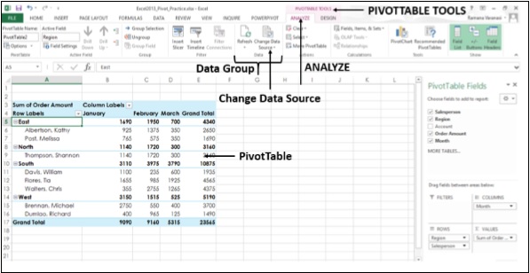
Step 1 − Click anywhere in the PivotTable. The PIVOTTABLE TOOLS appear on the ribbon, with an option named ANALYZE.

Step 2 − Click on the option - ANALYZE.

Step 3 − Click on Change Data Source in the Data group.

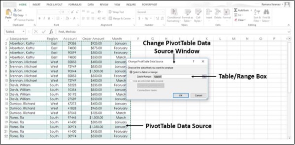
Step 4 − Click on Change Data Source. The current Data Source is highlighted. The Change PivotTable Data Source Window appears.

Step 5 − In the Table/Range Box, select the Table/Range you want to include.

Step 6 − Click OK.

Change to a Different External Data Source.

If you want to base your PivotTable on a different external source, it might be best to create a new PivotTable. If the location of your external data source is changed, for example, your SQL Server database name is the same, but it has been moved to a different server, or your Access database has been moved to another network share, you can change your current connection.

Step 1 − Click anywhere in the PivotTable. The PIVOTTABLE TOOLS appear on the Ribbon, with an ANALYZE option.

Step 2 − Click ANALYZE.

Step 3 − Click on Change Data Source in the Data Group. The Change PivotTable Data Source window appears.

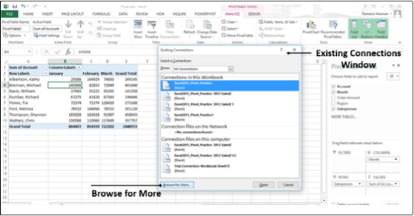
Step 4 − Click on the option Choose Connection.

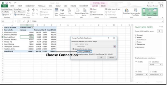
A window appears showing all the Existing Connections.

In the Show box, keep All Connections selected. All the Connections in your Workbook will be displayed.

Step 5 − Click on Browse for More…

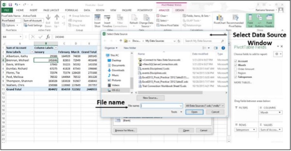
The Select Data Source window appears.

Step 6 − Click on New Source. Go through the Data Connection Wizard Steps.

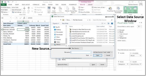
Alternatively, specify the File name, if your Data is contained in another Excel Workbook.

Delete a PivotTable

Step 1 − Click anywhere on the PivotTable. The PIVOTTABLE TOOLS appear on the Ribbon, with the ANALYZE option.

Step 2 − Click on the ANALYZE tab.

Step 3 − Click on Select in the Actions Group as shown in the image given below.

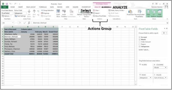
Step 4 − Click on Entire PivotTable. The entire PivotTable will be selected.

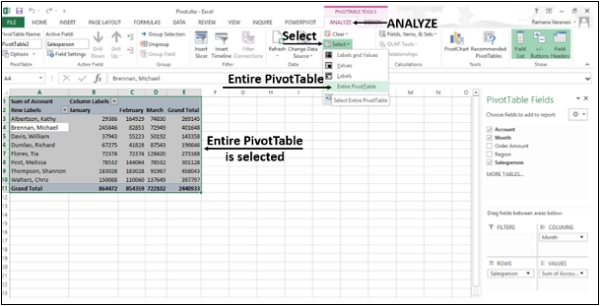
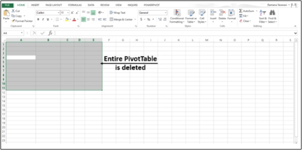
Step 5 − Press the Delete Key.

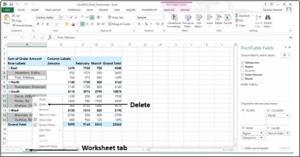
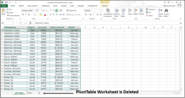
If the PivotTable is on a separate Worksheet, you can delete the PivotTable by deleting the entire Worksheet also. To do this, follow the steps given below.

Step 1 − Right-click on the Worksheet tab.

Step 2 − Click on Delete.

You get a warning message, saying that you cannot Undo Delete and might lose some data. Since, you are deleting only the PivotTable Sheet you can delete the worksheet.

Step 3 − Click on Delete.

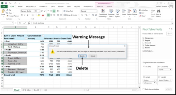
The PivotTable worksheet will be deleted.

Using the Timeline

A PivotTable Timeline is a box that you can add to your PivotTable that lets you filter by time, and zoom in on the period you want. This is a better option compared to playing around with the filters to show the dates.

It is like a slicer you create to filter data, and once you create it, you can keep it with your PivotTable. This makes it possible for you to change the time period dynamically.

Step 1 − Click anywhere in the PivotTable. The PIVOTTABLE TOOLS appear on the Ribbon, with ANALYZE option.

Step 2 − Click ANALYZE.

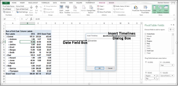
Step 3 − Click on Insert Timeline in the Filter group. An Insert Timelines Dialog Box appears.

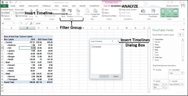
Step 4 − In the Insert Timelines dialog box, click on the boxes of the date fields you want.

Step 5 − Click OK.

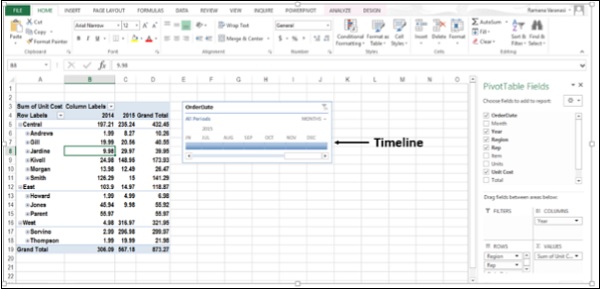
The timeline for your PivotTable is in place.

Use a Timeline to Filter by Time Period

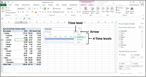
Now, you can filter the PivotTable using the timeline by a time period in one of four time levels; Years, Quarters, Months or Days.

Step 1 − Click the small arrow next to the time level-Months. The four time levels will be displayed.

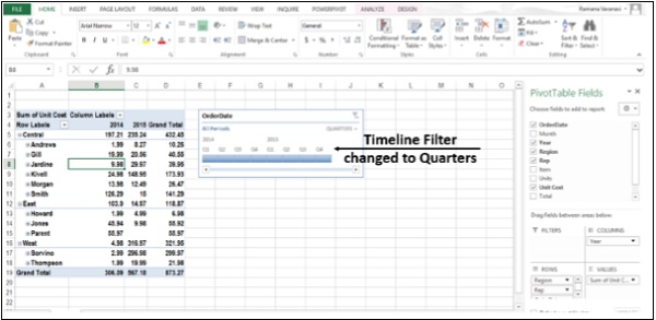
Step 2 − Click on Quarters. The Timeline filter changes to Quarters.

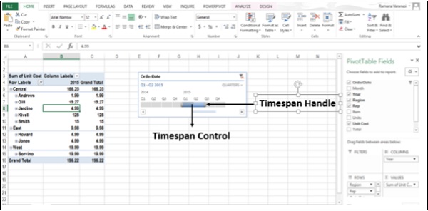
Step 3 − Click on Q1 2015. The Timespan Control is highlighted. The PivotTable Data is filtered to Q1 2015.

Step 4 − Drag the Timespan handle to include Q2 2015. The PivotTable Data is filtered to include Q1, Q2 2015.

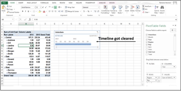
At any point of time, to clear timeline, click on the Clear Filter button.

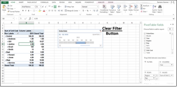
The timeline is cleared as shown in the image given below.

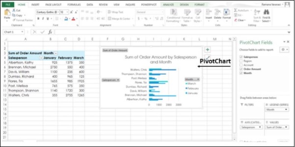
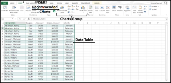
Create a Standalone PivotChart

You can create a PivotChart without creating a PivotTable first. You can even create a PivotChart that is recommended for your data. Excel will then create a coupled PivotTable automatically.

Step 1 − Click anywhere on the Data Table.

Step 2 − Click on the Insert tab.

Step 3 − In the Charts Group, Click on Recommended Charts.

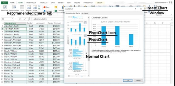
The Insert Chart Window appears.

Step 4 − Click on the Recommended Charts tab. The charts with the PivotChart icon in the top corner are PivotCharts.

Step 5 − Click on a PivotChart. A Preview appears on the Right side.

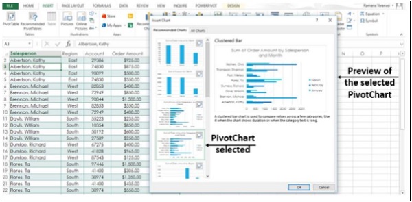
Step 6 − Click OK once you find the PivotChart you want.

Your standalone PivotChart for your Data is available to you.