Excel - PivotTable Recommendations

---

---

Excel 2013 has a new feature Recommended PivotTables under the Insert tab. This command helps you to create PivotTables automatically.

Step 1 − Your data should have column headers. If you have data in the form of a table, the table should have Table Header. Make sure of the Headers.

Step 2 − There should not be blank rows in the Data. Make sure No Rows are blank.

Step 3 − Click on the Table.

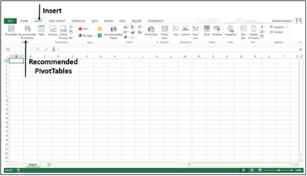
Step 4 − Click on Insert tab.

Step 5 − Click on Recommended PivotTables. The Recommended PivotTables dialog box appears.

Step 6 − Click on a PivotTable Layout that is recommended. A preview of that pivot table appears on the right–side.

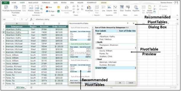
Step 7 − Double-click on the PivotTable that shows the data the way you want and Click OK. The PivotTable is created automatically for you on a new worksheet.

Create a PivotTable to analyze external data

Create a PivotTable by using an existing external data connection.

Step 1 − Click any cell in the Table.

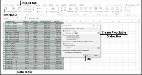
Step 2 − Click on the Insert tab.

Step 3 − Click on the PivotTable button. A Create PivotTable dialog box appears.

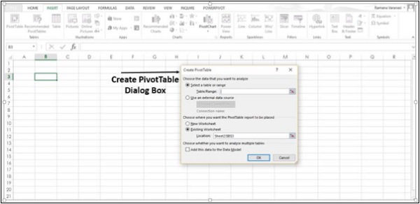
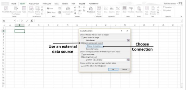
Step 4 − Click on the option Use an external data source. The button below that, ‘Choose Connection’ gets enabled.

Step 5 − Select the Choose Connection option. A window appears showing all the Existing Connections.

Step 6 − In the Show Box, select All Connections. All the available data connections can be used to obtain the data for analysis.

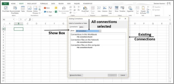
The option Connections in this Workbook option in the Show Box is to reuse or share an existing connection.

Connect to a new external data source

You can create a new external data connection to the SQL Server and import the data into Excel as a table or PivotTable.

Step 1 − Click on the Data tab.

Step 2 − Click on the From Other Sources button, in the Get External Data Group.

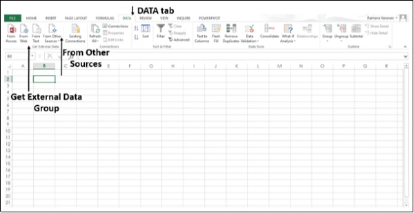
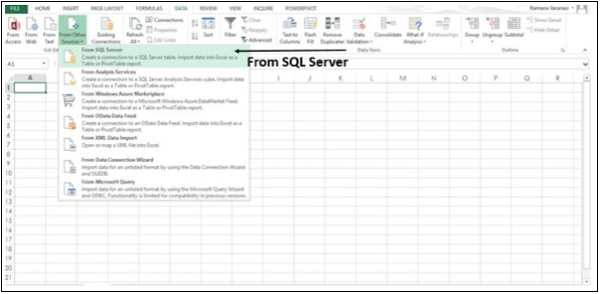
The options of External Data Sources appear as shown in the image below.

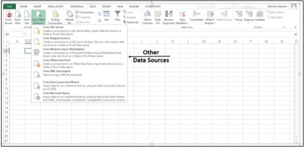
Step 3 − Click the option From SQL Server to create a connection to an SQL Server table.

A Data Connection Wizard dialog box appears.

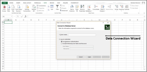
Step 4 − Establish the connection in three steps given below.

• Enter the database server and specify how you want to log on to the server.

• Enter the database, table, or query that contains the data you want.

• Enter the connection file you want to create.

Using the Field List option

In Excel 2013, it is possible to arrange the fields in a PivotTable.

Step 1 − Select the data table.

Step 2 − Click the Insert Tab.

Step 3 − Click on the PivotTable button. The Create PivotTable dialog box opens.

Step 4 − Fill the data and then click OK. The PivotTable appears on a New Worksheet.

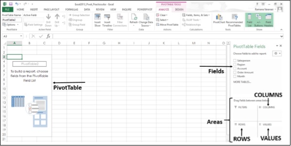
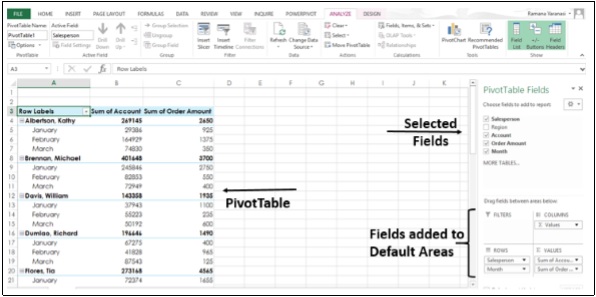
Step 5 − Choose the PivotTable Fields from the field list. The fields are added to the default areas.

The Default areas of the Field List are −

• Nonnumeric fields are added to the Rows area

• Numeric fields are added to the Values area, and

• Time hierarchies are added to the Columns area

You can rearrange the fields in the PivotTable by dragging the fields in the areas.

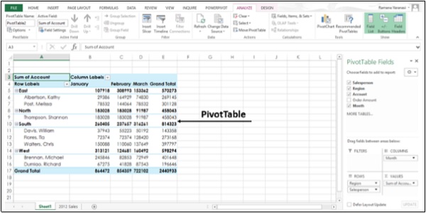
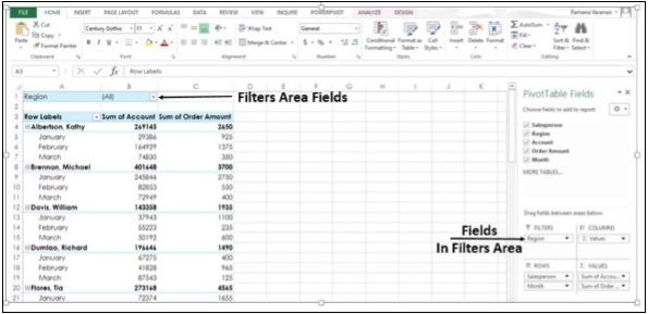
Step 6 − Drag Region Field from Rows area to Filters area. The Filters area fields are shown as top-level report filters above the PivotTable.

Step 7 − The Rows area fields are shown as Row Labels on the left side of the PivotTable.

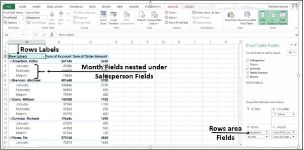
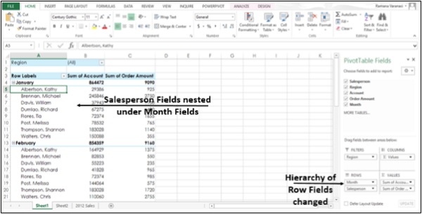
The order in which the Fields are placed in the Rows area, defines the hierarchy of the Row Fields. Depending on the hierarchy of the fields, rows will be nested inside rows that are higher in position.

In the PivotTable above, Month Field Rows are nested inside Salesperson Field Rows. This is because in the Rows area, the field Salesperson appears first and the field Month appears next, defining the hierarchy.

Step 8 − Drag the field - Month to the first position in the Rows area. You have changed the hierarchy, putting Month in the highest position. Now, in the PivotTable, the field - Salesperson will nest under Month fields.

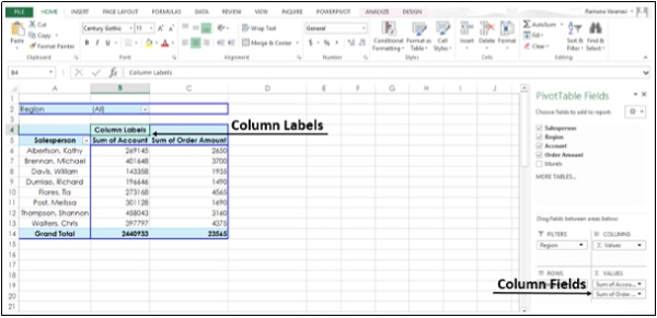
In a similar way, you can drag Fields in the Columns area also. The Columns area fields are shown as Column Labels at the top of the PivotTable.

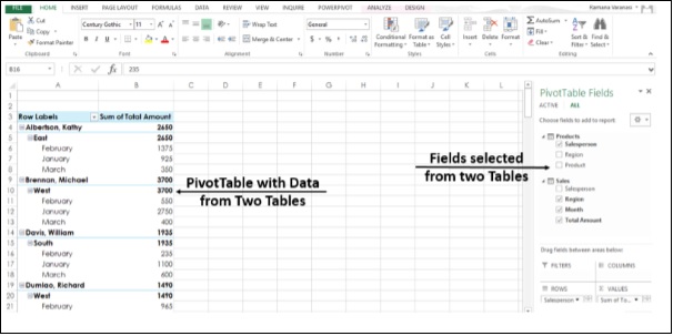
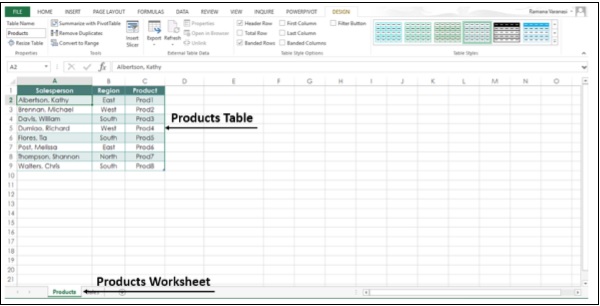
PivotTables based on Multiple Tables

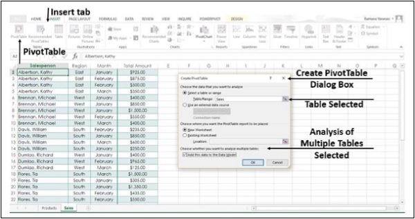
In Excel 2013, it is possible to create a PivotTable from multiple tables. In this example, the table ‘Sales’ is on one worksheet and table - ‘Products’ is on another worksheet.

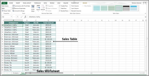
Step 1 − Select the Sales sheet from the worksheet tabs.

Step 2 − Click the Insert tab.

Step 3 − Click on the PivotTable button on the ribbon. The Create PivotTable dialog box,

Step 4 − Select the sales table.

Step 5 − Under “choose whether you want to analyze multiple tables”, Click Add this Data to the Data Model.

Step 6 − Click OK.

Under the PivotTable Fields, you will see the options, ACTIVE and ALL.

Step 7 − Click on ALL. You will see both the tables and the fields in both the tables.

Step 8 − Select the fields to add to the PivotTable. You will see a message, “Relationships between tables may be needed”.

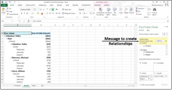
Step 9 − Click on the CREATE button. After a few steps for creation of Relationship, the selected fields from the two tables are added to the PivotTable.