
Article Categories
- All Categories
-
 Data Structure
-
 Networking
-
 RDBMS
RDBMS
-
 Operating System
-
 Java
Java
-
 MS Excel
-
 iOS
iOS
-
 HTML
HTML
-
 CSS
CSS
-
 Android
-
 Python
-
 C Programming
-
 C++
C++
-
 C#
C#
-
 MongoDB
-
 MySQL
MySQL
-
 Javascript
-
 PHP
PHP
-
 Economics & Finance
How to Copy and Paste Rows or Columns in Reverse Order in Excel?
When we have a list of elements in Excel and we want to arrange them in reverse order, it can be a complex and lengthy problem if we try to do it manually. We can make the order in reverse order easily if they are in a sorted list, but not in the case of unsorted lists. Read this tutorial to learn how you copy and paste rows or columns in reverse order in Excel.
Copy and Paste Column in Reverse Order in Excel
Here we will insert a VBA module and then run it to complete the task. Let's go over a simple procedure for copying and pasting columns in reverse order in Excel.
Step 1
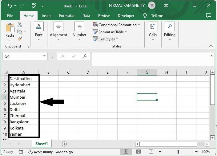
Consider any Excel sheet that contains a list of unsorted elements, similar to the image below.
We can use a VBA application to complete our process. To open the VBA application, right-click on the sheet name and select View Code.
Then, click Insert and select Module, and then type the following program1 into the text box, as shown in the image below.
Right click > View code > Insert > Module > Program 1
Program 1
Sub Flipvertically()
'Updated By Nirmal
Dim Rng As Range
Dim WorkRng As Range
Dim Arr As Variant
Dim i As Integer, j As Integer, k As Integer
On Error Resume Next
xTitleId = "Reverse the Order"
Set WorkRng = Application.Selection
Set WorkRng = Application.InputBox("Range", xTitleId, WorkRng.Address, Type:=8)
Arr = WorkRng.Formula
For j = 1 To UBound(Arr, 2)
    k = UBound(Arr, 1)
    For i = 1 To UBound(Arr, 1) / 2
        xTemp = Arr(i, j)
        Arr(i, j) = Arr(k, j)
        Arr(k, j) = xTemp
        k = k - 1
    Next
Next
WorkRng.Formula = Arr
End Sub

Step 2
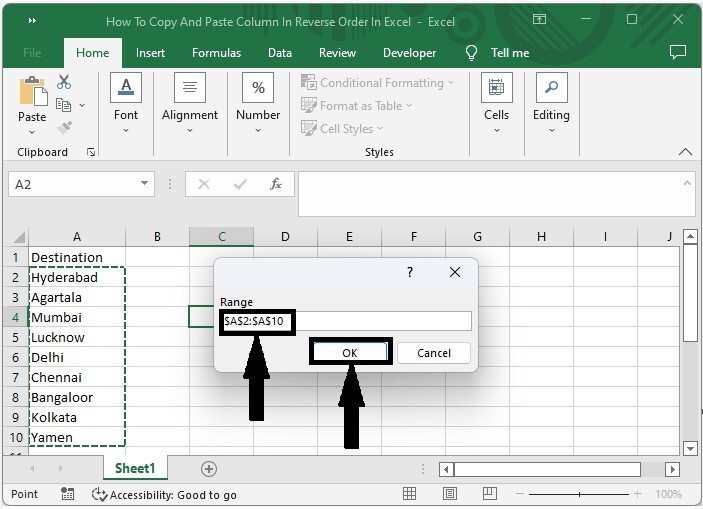
Now save the sheet as a macro-enabled worksheet, and in the vba application window, click F5 and select the range of cells you want to arrange, then click OK.
If we want to reverse the rows, we can use Program 2 instead of Program 1.
Program 2
Sub Fliphorizontally()
'Updated BY Nirmal
Dim Rng As Range
Dim WorkRng As Range
Dim Arr As Variant
Dim i As Integer, j As Integer, k As Integer
On Error Resume Next
xTitleId = "Reverse the order"
Set WorkRng = Application.Selection
Set WorkRng = Application.InputBox("Range", xTitleId, WorkRng.Address, Type:=8)
Arr = WorkRng.Formula
For i = 1 To UBound(Arr, 1)
    k = UBound(Arr, 2)
    For j = 1 To UBound(Arr, 2) / 2
        xTemp = Arr(i, j)
        Arr(i, j) = Arr(i, k)
        Arr(i, k) = xTemp
        k = k - 1
    Next
Next
WorkRng.Formula = Arr
End Sub
Conclusion
In this tutorial, we used a simple example to demonstrate how you can copy and paste rows or columns in reverse order in Excel.

2K+ Views
