How to lock and protect nonempty cells in Excel?

In this article, the user will learn the process of locking and protecting nonempty cells in Excel. Locking and protecting nonempty cells in a selected range with the "Protect Sheet" feature in spreadsheet applications like Excel facilitates an additional layer of security to prevent accidental or unauthorized modifications to important data. The example allows the user to lock and protect the nonempty cell, in the selected range, by using the available Excel features, and options.

Example: To Lock and protect all nonempty cells in a selected range with Protect Sheet

Step 1

To understand the process of locking and protecting nonempty cells within the selected range, the user first needs to consider a sample table, as shown below. In the below given table, will be using two columns. The month name is specified in the B column, while the C column compares the sale profit data value.

Step 2

Select the provided table, by clicking on B1 cell and selecting the table with data up to B12. In the Home tab, click on the “Editing” option, and select the option “Find & Select”. In the option, select the option “Go To Specials..” as highlighted below image −

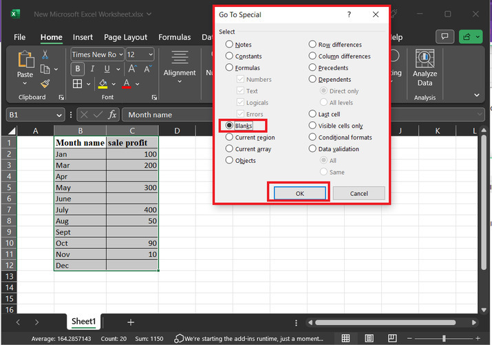
Step 3

The above step will display a “Go to Special”, dialog box. In the appeared dialog box, click on the option for “Blanks”. Finally, press the “OK” button.

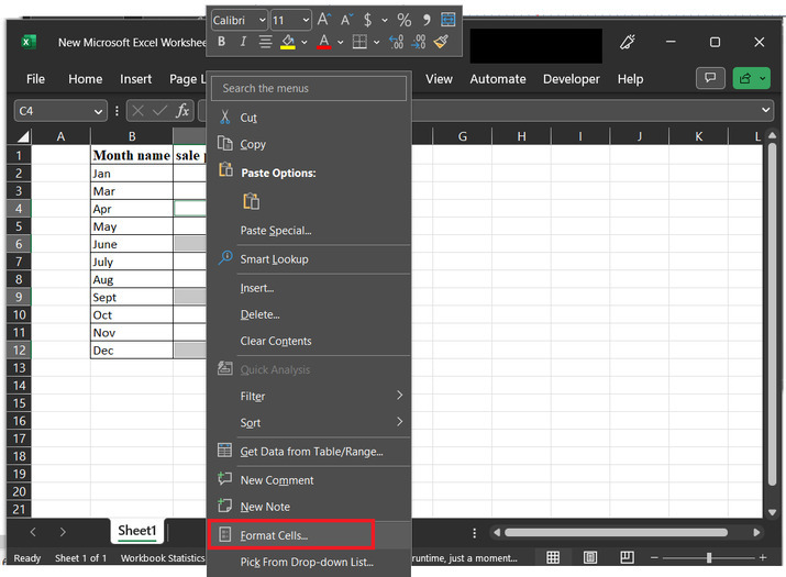
Step 4

The above step will select all the empty cells, as shown below. After that right click on any of the selected cells. this will display a list of available options. Among the displayed list of options, select the option with “Format Cells”.

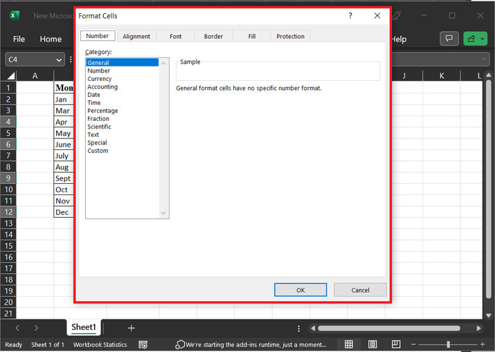
Step 5

The above step will display a dialog box for “Format Cells”. This option will display multiple tabs, here each tab has multiple options. Consider below given image snapshot for proper reference −

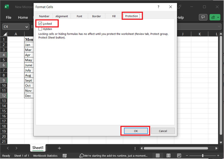
Step 6

Among all the available tabs, choose the “Protection” tab, and untick the “Locked” option. Finally, click on the “OK” button.

Step 7

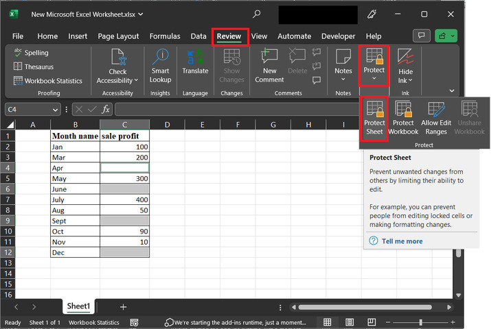
In the review tab, click on the “Protect” tab, and select the option for “Protect sheet” as shown below −

Step 8

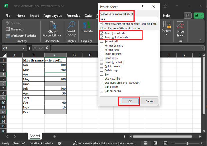
The above step will open a new dialog box, with the header “Protect Sheet”. In this dialog box, first, enter the password to make the sheet unprotected. In this example will assume that the password is “abc”. Please note that users can use any desirable password. But, make sure to remind the user password, as to make any change or to unprotect the sheet, the user needs this password only. After that select both first two options “Select locked cells” and “Select unlocked cells”. Finally, click on the “OK” button.

Step 9

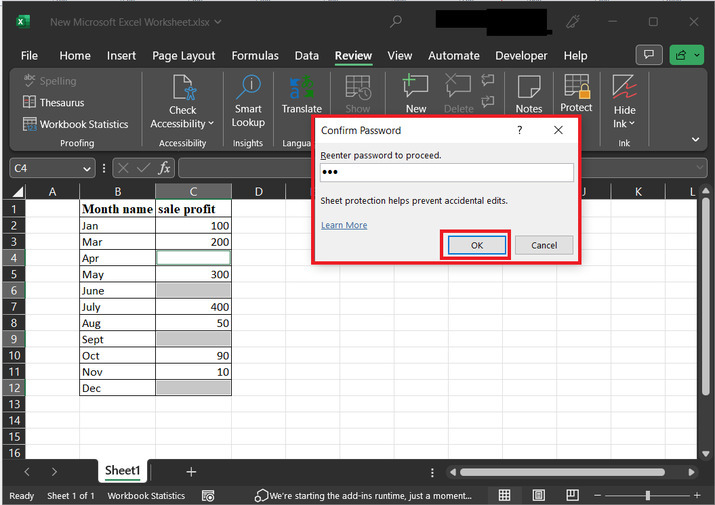
This will open a “Confirm Password” dialog box. This dialog box will allow the user to enter the password again, and click on the “OK” button.

Step 10

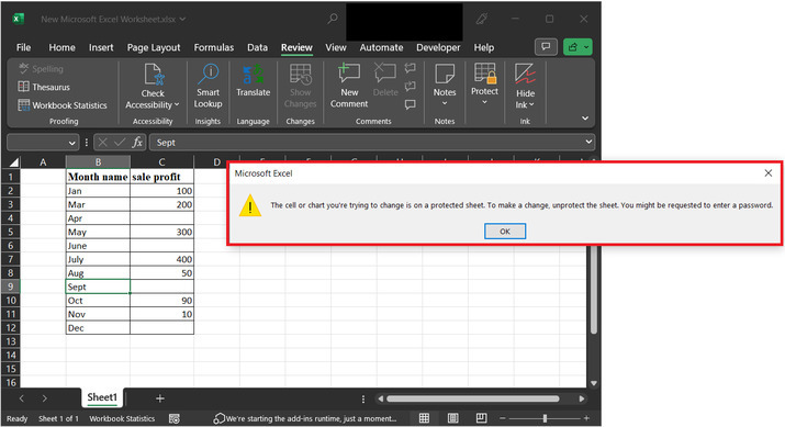
After that, try to click and edit any cell. in this example, the user is trying to modify the contents of the B9, cell. but this will display a dialog box, with the message, as depicted below. To remove the error message click on the “OK” button.

Conclusion

In this article, the user will learn the process of locking and protecting the non-empty cells of the Excel sheet. All the provided steps in the example are clear, precise, thorough, and fully relevant to the provided content.