
Article Categories
- All Categories
-
 Data Structure
-
 Networking
-
 RDBMS
RDBMS
-
 Operating System
-
 Java
Java
-
 MS Excel
-
 iOS
iOS
-
 HTML
HTML
-
 CSS
CSS
-
 Android
-
 Python
-
 C Programming
-
 C++
C++
-
 C#
C#
-
 MongoDB
-
 MySQL
MySQL
-
 Javascript
-
 PHP
PHP
-
 Economics & Finance
How To Create A Dynamic List Without Blank In Excel?
Excel is a powerful tool for managing and analyzing data, but one common issue users face is dealing with lists that contain empty cells. This can be especially frustrating when you're working with large datasets or trying to create charts and graphs. Fortunately, there is a simple solution: creating a dynamic list that automatically adjusts to exclude blank cells.
In this tutorial, we'll walk you through the steps for creating a dynamic list that eliminates blanks, allowing you to more easily work with and analyze your data. We'll cover everything from setting up your data range and creating a named range, to using the INDEX and COUNTA functions to build your dynamic list. By the end of this tutorial, you'll have a better understanding of how to create dynamic lists in Excel and how to eliminate blank cells, making your data management tasks more efficient and effective. So let's get started!
Create A Dynamic List Without Blank
Here we will first count the unique records and list them, then finally create the list using the data validation. So let us see a simple process to know how you can create a dynamic list without leaving any cells blank in Excel.
Step 1
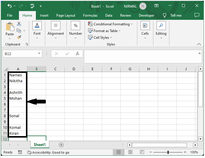
Consider an Excel sheet where you have a list of names with empty cells in between, similar to the below image.
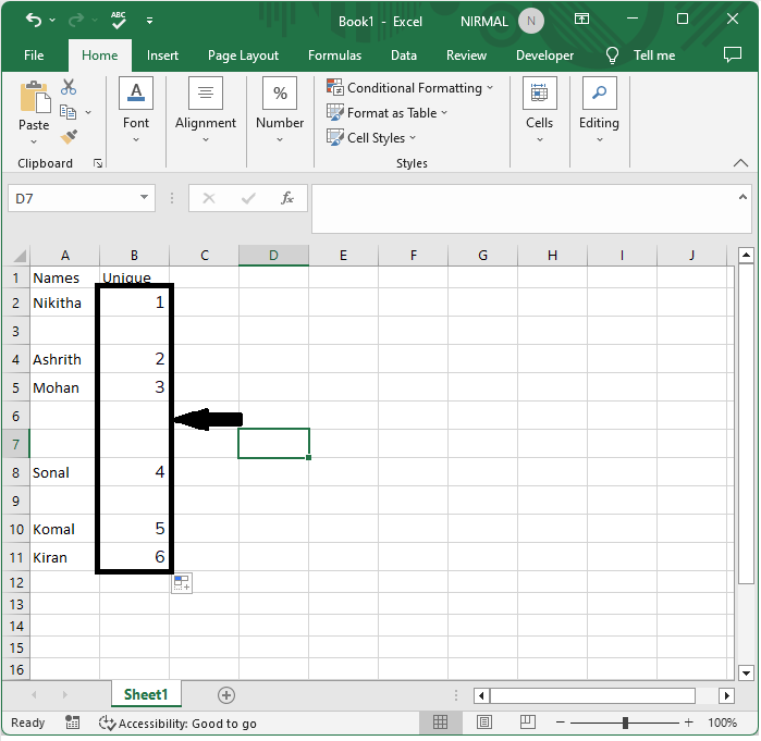
First, click on an empty cell, in our case cell B2, and enter the formula as
=IF(A2="","",MAX(B$1:B1)+1) and click enter to get the first value.
Empty cell > Formula > Enter.

Step 2
Then drag down from the first value to number all the records.
Step 3
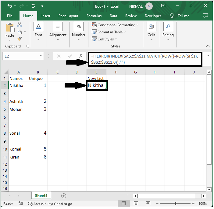
Now again click on an empty cell, in this case cell E2, and enter the formula as =IFERROR(INDEX($A$2:$A$11,MATCH(ROW()-ROW($F$1),$B$2:$B$11,0)),"") and click enter.
Empty cell > Formula > Enter.
Step 4
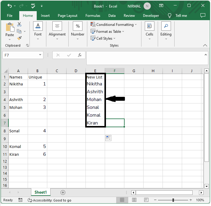
Then drag down the result form to list all the values.
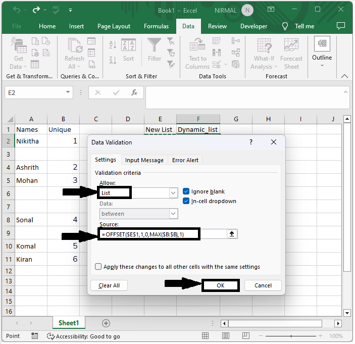
Step 5
Finally, click on an empty cell, then click on data and select data validation to open the pop-up. Then change the allow list and range to =OFFSET($E$1,1,0,MAX($B:$B),1) and click on to complete the task.
Empty cell > Data > Data Validation > List > Formula > Ok.
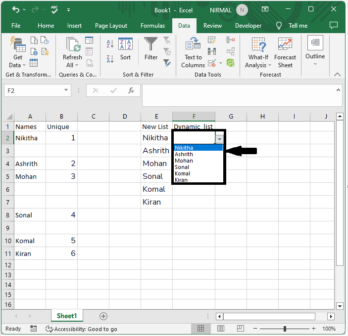
Then we can finally see that the data validation list will be created successfully.
Conclusion
In this tutorial, we have used a simple example to demonstrate how you can create a dynamic list without blank cells in Excel to highlight a particular set of data.

3K+ Views
