
Article Categories
- All Categories
-
 Data Structure
-
 Networking
-
 RDBMS
RDBMS
-
 Operating System
-
 Java
Java
-
 MS Excel
-
 iOS
iOS
-
 HTML
HTML
-
 CSS
CSS
-
 Android
-
 Python
-
 C Programming
-
 C++
C++
-
 C#
C#
-
 MongoDB
-
 MySQL
MySQL
-
 Javascript
-
 PHP
PHP
-
 Economics & Finance
How to Create a Searchable Drop Down List in Excel?
Powerful tools like Excel are frequently used for data management, organisation, and analysis. Making drop-down lists, which provide users specified alternatives to choose from and guarantee data quality and consistency, is one of its primary characteristics. A typical drop-down list is useful, but what if you could make it even better by making it searchable? Think about how much easier it would be to discover the necessary option by inputting a few characters as opposed to scrolling through a long list.
We'll walk you through the steps of making a searchable drop-down list in Excel in this tutorial. You may add a search feature to your drop-down lists by using the built-in functions and data validation strategies of Excel by following the step-by-step instructions provided here. Whether you're a novice or a seasoned Excel user, this course will give you the skills you need to improve your productivity and streamline the data entering process.
Create a Searchable Drop Down
Here we will first insert an ActiveX Control Combo box, then use some formulas, and finally use VBA code to complete the task. So let us see a simple process to learn how you can create a searchable drop-down list in Excel.
Step 1
Consider an Excel sheet where you have a list of items similar to the below image.
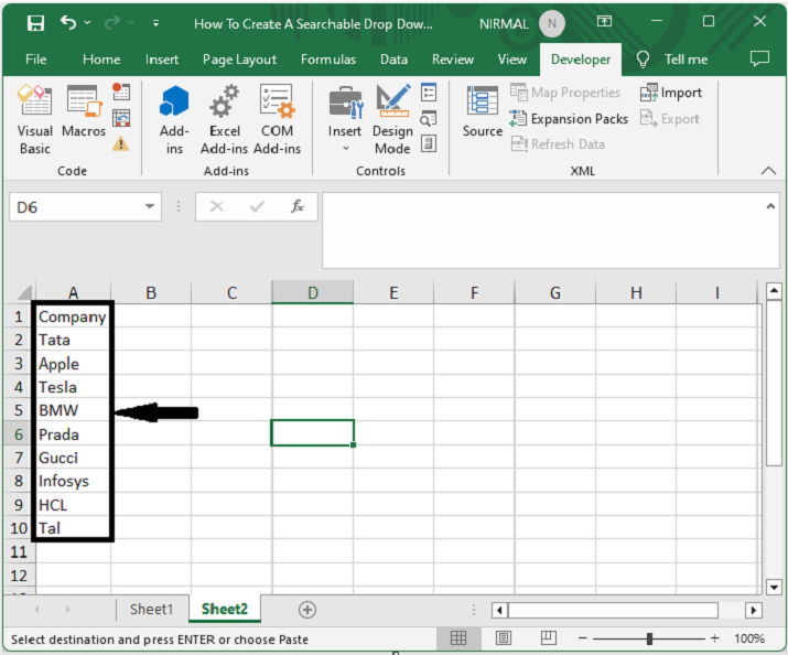
Now click on formulas and click on Define Name, then enter List as Name, and for Source, select the range of cells in the list, and click Ok.

Step 2
First, click on developer, then click on insert, then click on insert, and select Combo Box under ActiveX controls.
Developer > Insert > Combo Box.
Step 3
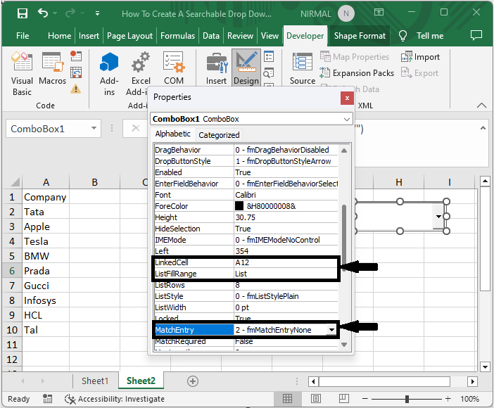
Then draw a box of the required size. Then right-click on the box, select Properties, and make the below changes.
First, select AutoWordSelect to False, then enter cell A12 in the linked cell field, then select 2-fmMatchEntryNone in the MatchEntry Field, enter List in the ListFillRange field, and finally close the properties.
Right click > Properties > AutoWordSelect > Linked Cell > MatchEntry > ListFillRange > Close.
Step 4
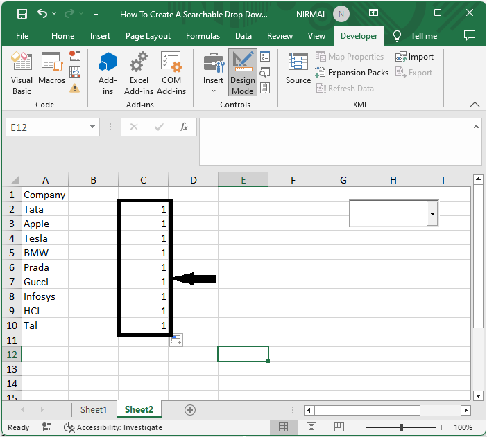
Then exit the Design mode, enter a letter in cell A12 and click on cell C2, and enter the formula as =--ISNUMBER(IFERROR(SEARCH($A$12,A2,1),"")) and click enter. Then drag down using the autofill handle.
Empty cell > Formula > Enter.
Step 5
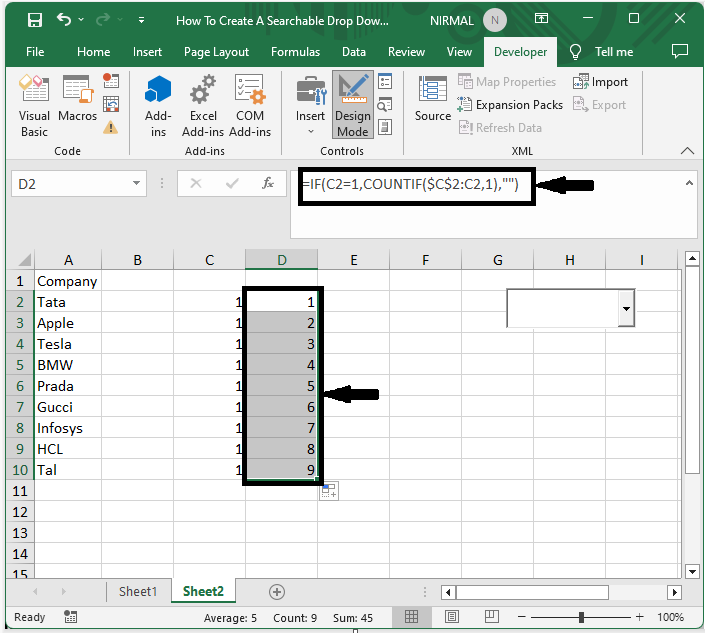
Then in cell D2, enter the formula as =IF(C2=1,COUNTIF($C$2:C2,1),""), click enter, and drag using the autofill handle.
Empty cell > Formula > Enter.
Step 6
Then in cell E2, enter the formula as
=IFERROR(INDEX($A$2:$A$9,MATCH(ROWS($D$2:D2),$D$2:$D$9,0)),"") and drag down using the auto fill handle.
Empty cell > Formula > Enter.
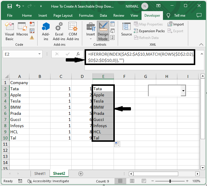
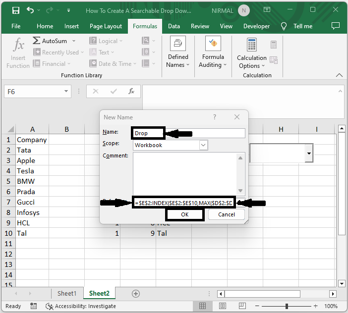
Step 7
Then click on Define Name under formulas and enter name as Drop and refer to it as =$E$2:INDEX($E$2:$E$10,MAX($D$2:$D$10),1) and click Ok.
Formulas > New Name > Name > Refers To > Ok.
Step 8
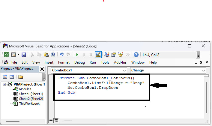
Then right-click on the combo box and select View Code." Then replace the existing code with the below code.
Right click > View code > Replace Code.
Code
Private Sub ComboBox1_GotFocus()
	ComboBox1.ListFillRange = "Drop"
	Me.ComboBox1.DropDown
End Sub
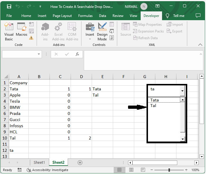
Step 9
Then, finally, use Alt + Q to close the VBA. Then searching will be possible.
Conclusion
In this tutorial, we have used a simple example to demonstrate how you can create a searchable drop-down list in Excel to highlight a particular set of data.

4K+ Views
