How to add color to a drop-down list in Excel?

Color can be a powerful element in an Excel drop down list, and it's easier to incorporate than you may think. We can add conditional formatting rules to the cell containing the drop-down list. Learn how to provide visual clues by adding a new list and validation control, followed by conditional format rules.

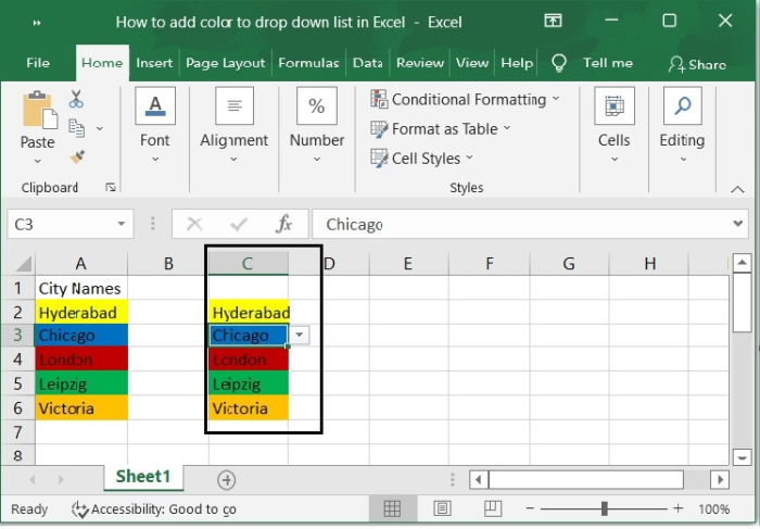
For example, I have created a drop-down list of city names; when I select "Hyderabad", I want the cell to be colored Yellow automatically, and when I select "Chicago", I want the cell to be colored Blue, as shown in the screenshot below.

First, Create a Drop-Down List

Let’s understand step by step with an example.

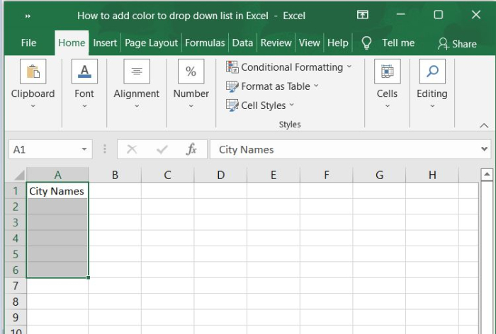
Step 1

Make a list of data and choose a range into which to place the drop-down list values. In this scenario, I positioned the drop-down list in the range A2:A6, as shown in the screenshot −

Step 2

To see a screenshot, select Data > Data Validation > Data Validation.

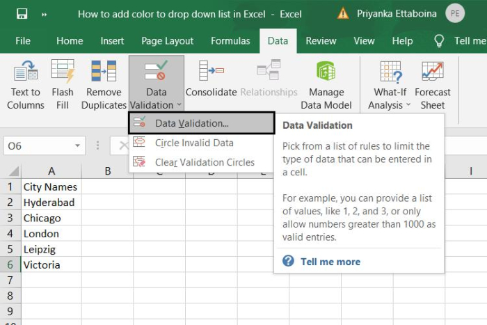
Step 3

Additionally, in the "Data Validation" dialogue box, click the Settings tab and select List from the Allow drop down list.

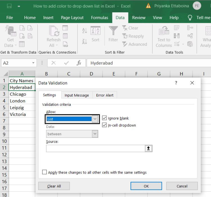
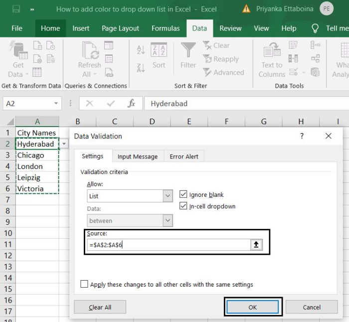
Step 4

Now select the Source option and click OK.

Step 5

Now, we can see the Drop-Down list below.

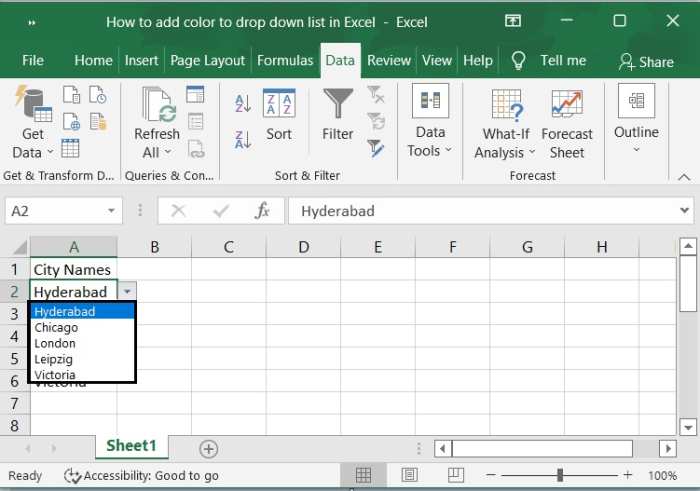
Now, we can add a color to the drop-down list.

A Color-coded Drop-Down List with Conditional Formatting

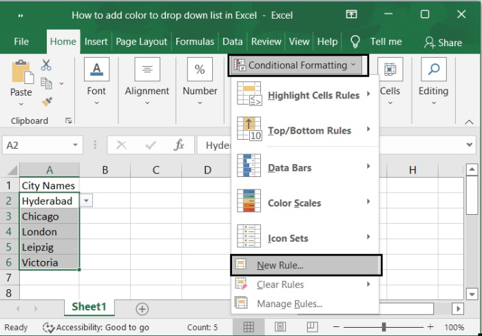
Step 1

Mark your drop-down cells, which in this case are in column A, and go to Home > Conditional Formatting then select New Rule.

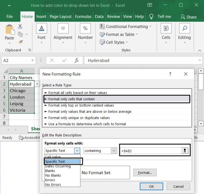
Step 2

Now click the New Rule option. Then you can see the New Formatting Rule dialog box, click the Format only cells that contain option under the Select a Rule Type section. Under the Format only cells with section, choose Specific Text from the first drop-down list and containing from the second drop-down list. Then, click the doc button 1 button to choose the value you want to format with a certain color, see screenshot.

Step 3

Then click the Format button.

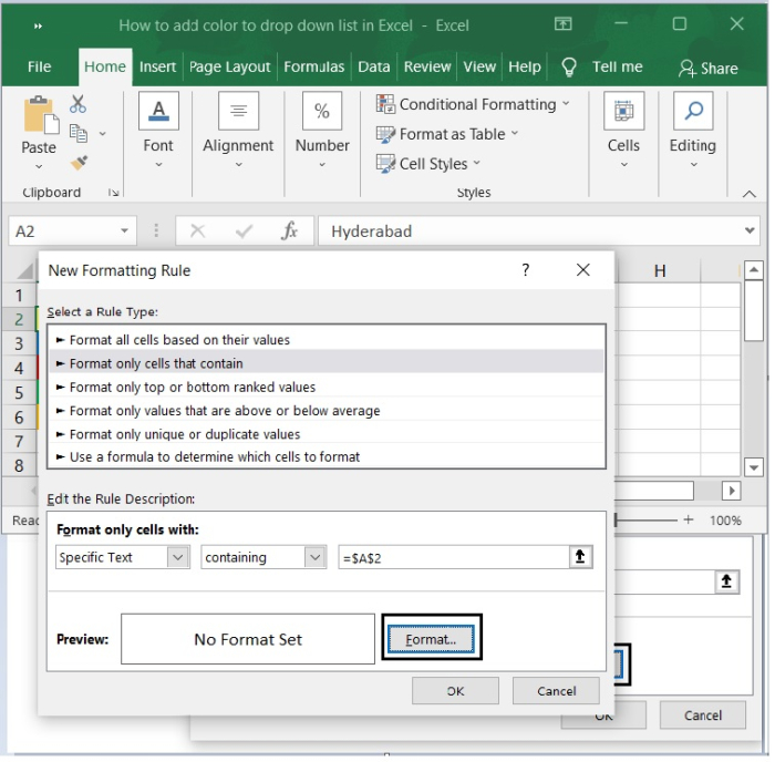
Step 4

And then click the Fill tab, choose a colour you like.

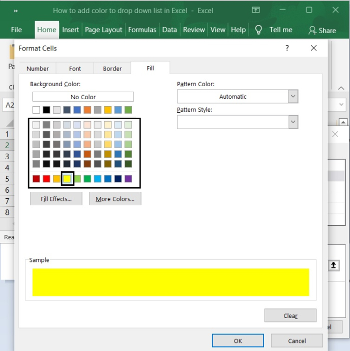
And then click OK to close the dialogs, repeat steps 1 to 4 for each other drop down selection.

Step 5

Now, click Conditional Formatting, then click Manage Rules, select the cell range to Apply the Conditional Formatting.

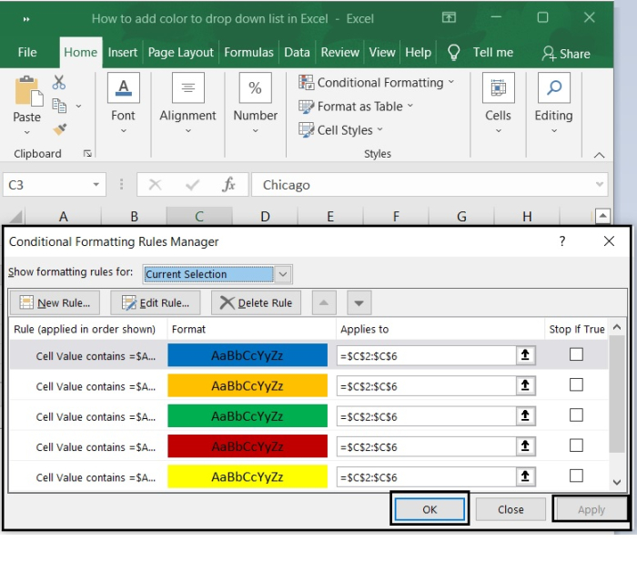
Step 6

Once you've set the colors for the values, you can choose any value from the drop-down menu and the cell will automatically change to the colour you chose.

Conclusion

In this tutorial, we explained with an example how to add color to a drop-down list using Conditional Formatting by creating and managing conditional formatting rules.