How To Create Drop Down List But Show Different Values In Excel?

Microsoft Excel is a powerful tool for data management and analysis, offering a wide range of features and functionalities to streamline your workflow. One such feature is the drop-down list, which allows you to select values from a predefined set of options. By default, a drop-down list in Excel displays the same values for each cell. However, in some cases, you may need to display different values for each cell, depending on certain criteria or conditions. In this tutorial, we will explore how to create a dynamic drop-down list in Excel that shows different values based on the data in each cell. Whether you're a beginner or an experienced Excel user, this tutorial will provide you with the step-by-step guidance you need to create and customize your own dynamic drop-down lists in Excel.

Create Drop Down List But Show Different Values

Here, we will first create a data validation list and then insert the VBA code to complete the task. So let us see a simple process to know how you can create a drop-down list but show different values in Excel.

Step 1

Consider an Excel sheet where the data is similar to the below image.

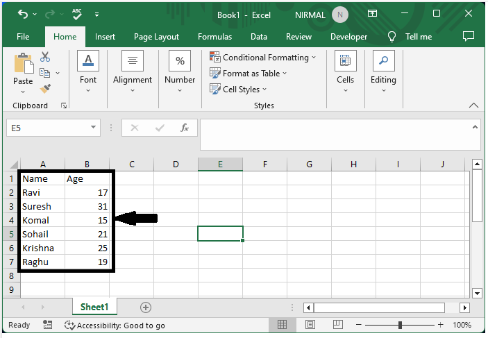
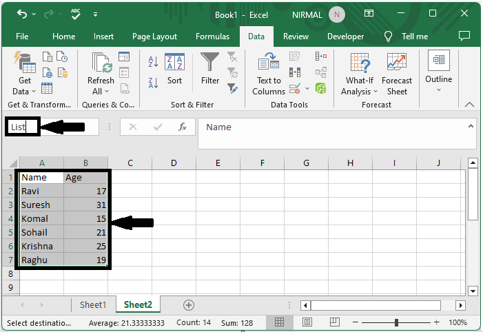
First, select the range of cells, then click on the name box, enter the name as a dropdown, and click enter.

Step 2

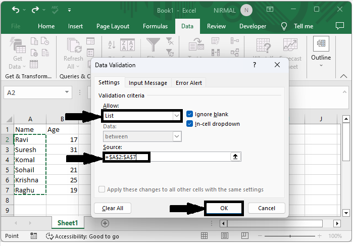
Then click on an empty cell where you want to insert the drop-down list, then click on data and select data validation. Then set allow to list and source to the names, and click OK.

Step 3

Now right-click on the sheet name and select view code to open the VBA application, then copy the below-mentioned code into the text box as shown in the below image.

Code

Private Sub Worksheet_Change(ByVal Target As Range)
   selectedNa = Target.Value
   If Target.Column = 4 Then
      selectedNum = Application.VLookup(selectedNa, ActiveSheet.Range("List"), 2, False)
      If Not IsError(selectedNum) Then
         Target.Value = selectedNum
      End If
   End If
End Sub

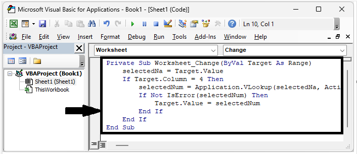
Then the final result will be similar to the below image.

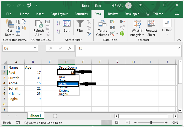
Conclusion

In this tutorial, we have used a simple example to demonstrate how you can create a drop-down list but show different values in Excel to highlight a particular set of data.