How to remove (temporarily hide) conditional formatting when printing in Excel?

In the article, we may go to remove or hide temporary the conditional formatting once the users will print the data they want to print from random numbers in the worksheet that the users have to analyze the data or random numbers to remove the conditional formatting. The users must remove or hide the formatting by using data validation and conditional formatting rules. Incorrect entries, fault is determined by using Data Validation concept. It also reduces the user’s time to find the error resided in the dataset.

Example 1: By Using Data Validation

Step 1

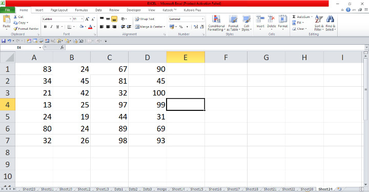
Deliberate the Excel worksheet. Open the Microsoft Excel sheet and insert the data from the cells A1 to B10 as you need as shown below.

Step 2

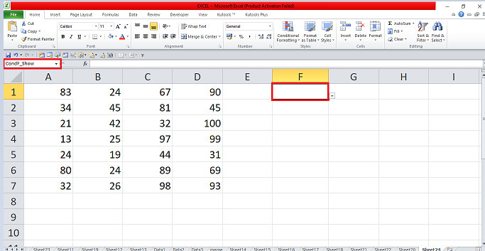
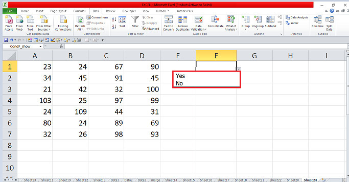
In the Excel sheet, locate the pointer and select the cell F1 and place the pointer in the Name box then type CondF_Show and press Enter key that will show the drop-down arrow in the selected cell as shown below.

Step 3

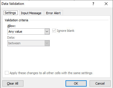
In the Excel sheet, select the cell and locate the pointer within the ribbon dataset. On the Data tab, place the pointer and connect to the Data Validation tab which has the drop-down menu. In the menu, choose and link to the option Data Validation tab in the Data Tools group that will open the dialog box as shown below.

Step 4

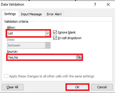
In the dialog box, place the pointer and select the option List in the Allow drop-box then place the pointer and type Yes, No in the Source input type then click on the OK button that will show the Yes and No values in the cell F1 as shown below.

Step 5

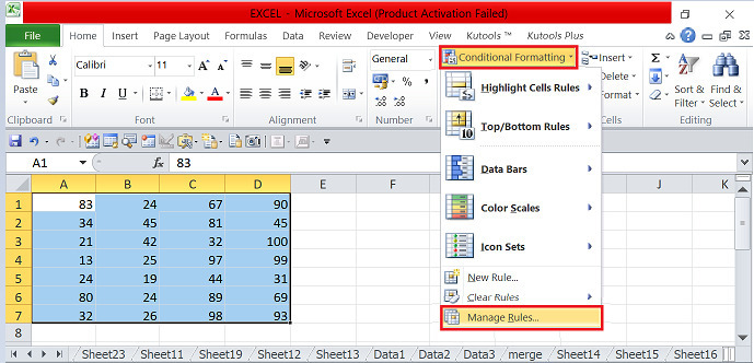
In the Excel sheet, select all the cells and locate the pointer within the ribbon dataset. There are various tabs comprised within the top corner. Place the pointer within the Home tab and connect to the tab that has countless options encompassed. On the Home tab, place the pointer and connect to the Conditional Formatting tab that has the drop-down menu. In the menu, choose and link to the option Manage Rules tab in the Styles group that will open the dialog box as shown below.

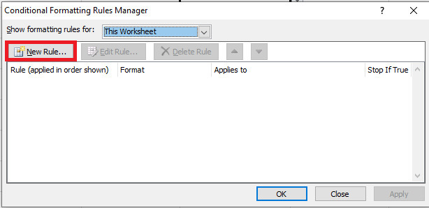
Step 6

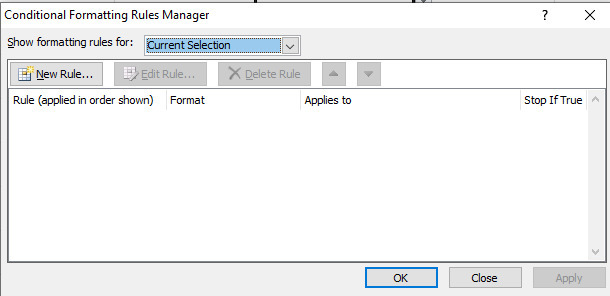
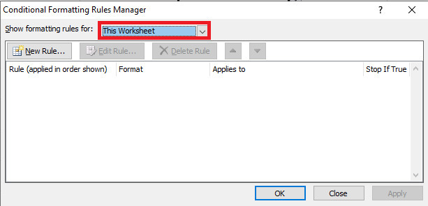
In the dialog box, locate the cursor and select the option This worksheet in the Show formatting rules for drop-box then click on the New Rule tab to open the dialog box as shown below.

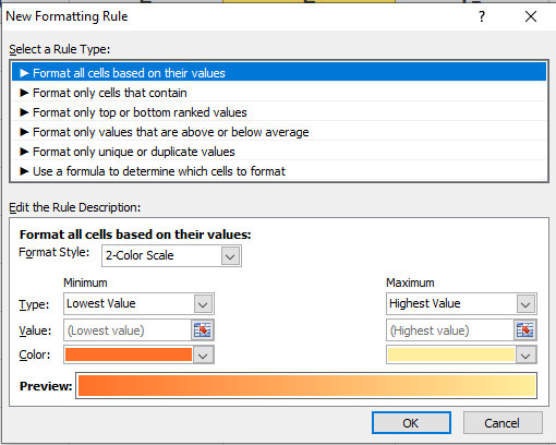
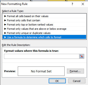
Step 7

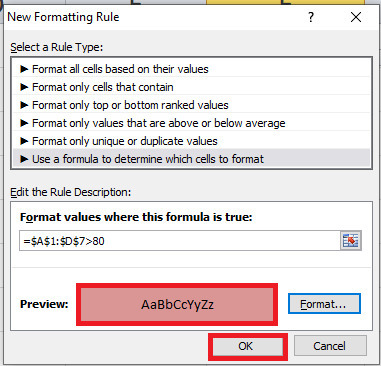
In the dialog box, place the pointer and select Use a formula to determine which cells to format to enter the formula as shown below.

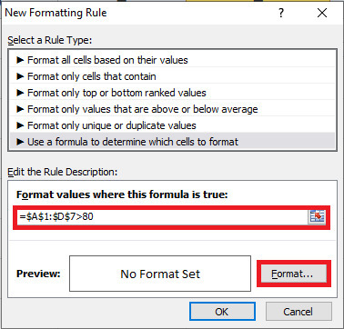
Step 8

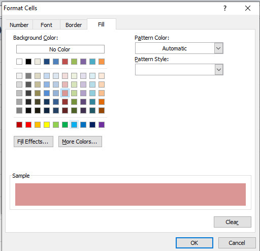
In the dialog box, place the pointer in the sheet and select all the cells then type >80 to enter the formula then click on the Format button that will open the box. In the box, select the Fill tab then select any color to highlight the data then click on the ok button as shown below.

Step 9

In the dialog box, click on the OK button that will open the dialog box Conditional formatting rules Manager.

Step 10

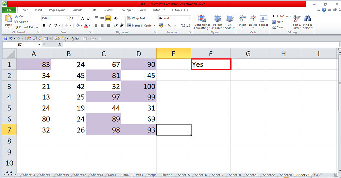
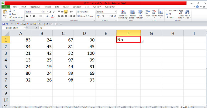
In the dialog box click on the OK button that will show the selected values highlighted if the users must select the Yes option. Only 80 above values are highlighted that we have used with the Yes option. If the users will select the No option then the highlighted areas are removed or hide or removed the conditional formatting as shown below.

The step-by-step explanation is demonstrated in this article to remove or hide the conditional formatting by using the conditional formatting rule to enter the formula which we want to highlight. We used the function CondF_Show in the Name box to show the highlighted values and hide the conditional formatting that is present in the sheet. The users created random numbers that will enter and locate the formula if we remove and highlight the values. They have to practice the vital choices from the ribbon and update the data.