How to compare adjacent cells with Conditional Formatting icon sets in Excel?

Conditional format icons are used for better data visualization in excel. It gives an instant data analysis to the viewer. For example, Icon sets can be used in the following scenarios; comparison of greater than, less than and equals to data item, comparison of highest temperature and lowest temperature, comparison between price inflation etc. In this article we will learn how to put icons instead of number while comparing adjacent cells of a rows or columns in an excel file by using the following methods −

• Compare adjacent column cells with Conditional Formatting icon set in Excel

• Compare adjacent rows cells with Conditional Formatting icon set in Excel

Compare Adjacent Column Cells with Conditional Formatting Icon Set

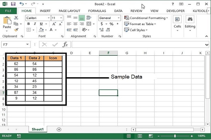
Step 1 − We have taken the following sample data to compare the values of Data 1 and Data 2 as less than, greater than or equals to. The final output icon will be visible under Icon column.

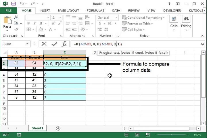
Step 2 − Enter the following formula in the second row of Icon column and drag the same till the last row till which you want to compare the data.

=IF(A2>B2, 0, IF(A2<B2, 2,1))

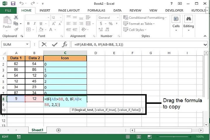
Step 3 − After dragging the formula till the last row, the following output will be displayed. Here, 0 means Data 1 is greater than Data 2, 1 means both values are equal, 2 means Data 1 is less than Data 2.

Formula Syntax Description

Argument	Description
IF(logical_test, {value_if_true},{value_if_false}	• Logical_test specifies the condition basis which the data needs to be rendered. • Value_if_true specifies the value that shall be returned if the condition satisfies. • Value_if_false specifies the value that shall be returned if the condition does not satisfy.

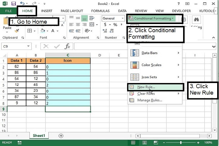
Step 4 − Now select the Icon column and go to Home / Conditional Formatting / New Rule as shown in the below screenshot to replace the 0,1,2 from icons.

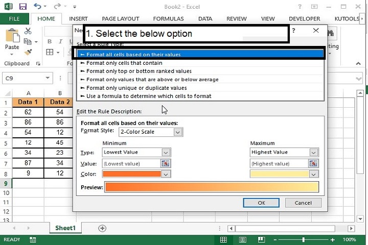
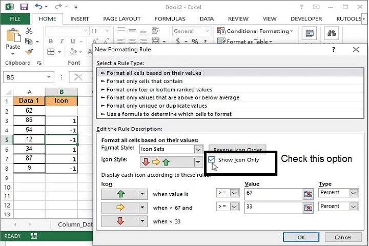
Step 5 − The new Formatting Rule prompt will open. Follow the below steps −

Select Format all cells based on their values option in the Select a Rule Type list box;

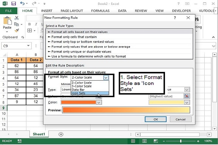
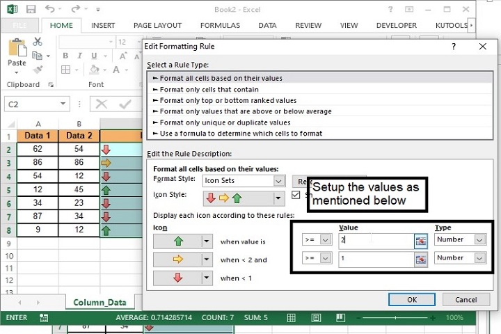
Step 6 − Under the Edit Rule Description section, select Icon Style against Format Style drop-down

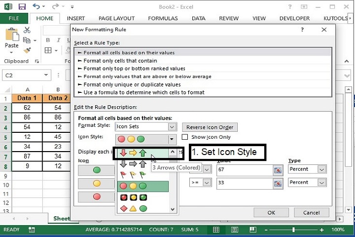
Step 7 − Now select the colored arrow icon against Icon Style.

Step 8 − Check the checkbox of Show Icon Only.

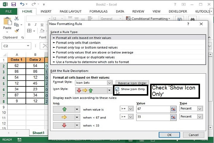
Step 9 − Now change the Type as Number and Value as 2 against the field >= and as 1 against the field >= and click OK. The Final output will be as shown below.

Compare Adjacent Rows Cells with Conditional Formatting Icon Set

To compare the values of two adjacent rows and using conditional formatting icons, follow the below steps.

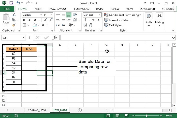
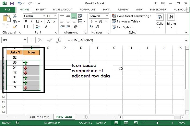
Step 1 − Following is the sample data for row comparison.

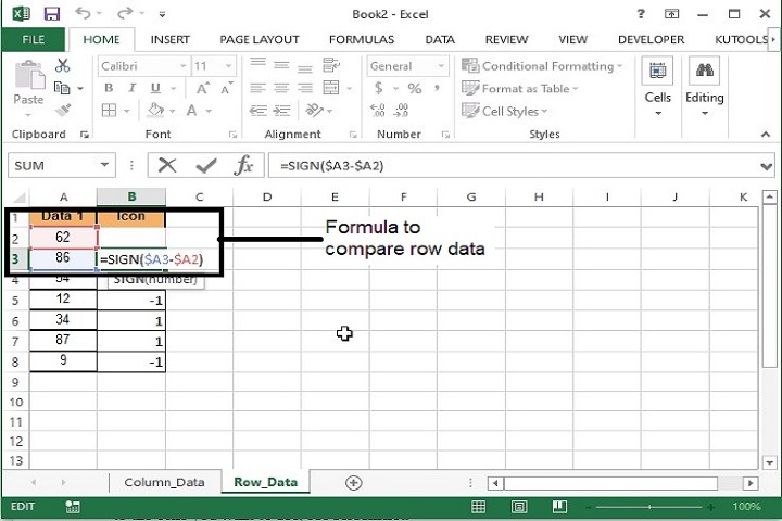
Step 2 − Now, enter the following formula under the icon column as shown below, after leaving the first data of the row.

=SIGN($A3-$A2)

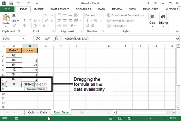
Step 3 − Now drag the formula to the last row to compare the all values.

Formula Syntax Description

Argument	Description
Sign(Number}	The SIGN formula in Excel displays only three results: +1, 0, and -1. If the number is greater than zero, the Excel SIGN formula will return 1. If the number equals zero, the SIGN formula in Excel will return 0. If the number is more than zero, the SIGN formula in Excel will return -1.

Step 4 − Now, follow the below steps to replace the numbers with icons.

Step 5 − Now select the Icon column and go to Home / Conditional Formatting / New Rule as shown in the below screenshot to replace the 0, 1, and -1 from icons.

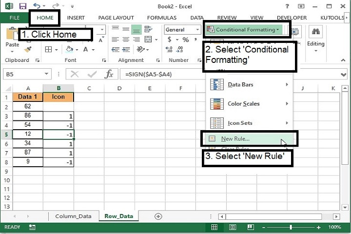
Step 6 − The new Formatting Rule prompt will open. Follow the below steps: Select Format all cells based on their values option in the Select a Rule Type list box;

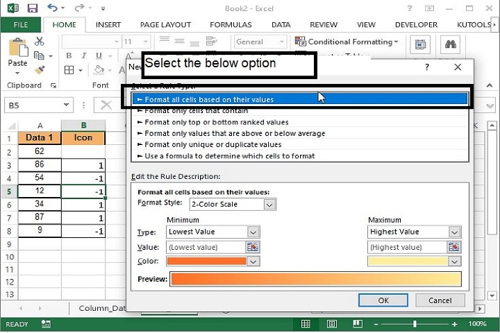
Step 7 − Under the Edit Rule Description section, select Icon Style against Format Style drop-down.

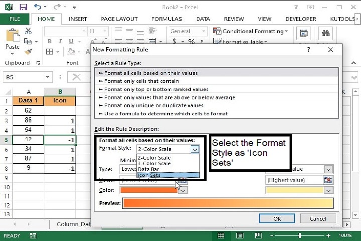
Step 8 − Now select the colored arrow icon against Icon Style.

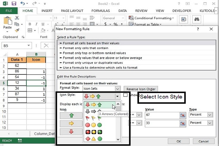
Step 9 − Check the checkbox of Show Icon Only.

Step 10 − Now change the Type as Number, change the symbol (>=) to (>) against “When value is” field.” Also, update the value as 0 under Value column against both value fields.

Step 11 − Finally click OK. The expected icons will be available under Icon column.

Conclusion

Hence, in this article we have learned how to replace comparison output data with conditional formatting icon sets. This method can be applied to non-adjacent cells as well by replacing the cell address in the formula. Keep exploring and keep learning excel for new features.