
- Excel - Home
- Excel - Getting Started
- Excel - Explore Window
- Excel - Backstage
- Excel - Entering Values
- Excel - Move Around
- Excel - Save Workbook
- Excel - Create Worksheet
- Excel - Copy Worksheet
- Excel - Hiding Worksheet
- Excel - Delete Worksheet
- Excel - Close Workbook
- Excel - Open Workbook
- Excel - Merge Workbooks
- Excel - File Password
- Excel - File Share
- Excel - Emoji & Symbols
- Excel - Context Help
- Excel - Insert Data
- Excel - Select Data
- Excel - Delete Data
- Excel - Move Data
- Excel - Rows & Columns
- Excel - Copy & Paste
- Excel - Find & Replace
- Excel - Spell Check
- Excel - Zoom In-Out
- Excel - Special Symbols
- Excel - Insert Comments
- Excel - Add Text Box
- Excel - Shapes
- Excel - 3D Models
- Excel - CheckBox
- Excel - Add Sketch
- Excel - Scan Documents
- Excel - Auto Fill
- Excel - SmartArt
- Excel - Insert WordArt
- Excel - Undo Changes
- Formatting Cells
- Excel - Setting Cell Type
- Excel - Move or Copy Cells
- Excel - Add Cells
- Excel - Delete Cells
- Excel - Setting Fonts
- Excel - Text Decoration
- Excel - Rotate Cells
- Excel - Setting Colors
- Excel - Text Alignments
- Excel - Merge & Wrap
- Excel - Borders and Shades
- Excel - Apply Formatting
- Formatting Worksheets
- Excel - Sheet Options
- Excel - Adjust Margins
- Excel - Page Orientation
- Excel - Header and Footer
- Excel - Insert Page Breaks
- Excel - Set Background
- Excel - Freeze Panes
- Excel - Conditional Format
- Excel - Highlight Cell Rules
- Excel - Top/Bottom Rules
- Excel - Data Bars
- Excel - Color Scales
- Excel - Icon Sets
- Excel - Clear Rules
- Excel - Manage Rules
- Working with Formula
- Excel - Formulas
- Excel - Creating Formulas
- Excel - Copying Formulas
- Excel - Formula Reference
- Excel - Relative References
- Excel - Absolute References
- Excel - Arithmetic Operators
- Excel - Parentheses
- Excel - Using Functions
- Excel - Builtin Functions
- Excel Formatting
- Excel - Formatting
- Excel - Format Painter
- Excel - Format Fonts
- Excel - Format Borders
- Excel - Format Numbers
- Excel - Format Grids
- Excel - Format Settings
- Advanced Operations
- Excel - Data Filtering
- Excel - Data Sorting
- Excel - Using Ranges
- Excel - Data Validation
- Excel - Using Styles
- Excel - Using Themes
- Excel - Using Templates
- Excel - Using Macros
- Excel - Adding Graphics
- Excel - Cross Referencing
- Excel - Printing Worksheets
- Excel - Email Workbooks
- Excel- Translate Worksheet
- Excel - Workbook Security
- Excel - Data Tables
- Excel - Pivot Tables
- Excel - Simple Charts
- Excel - Pivot Charts
- Excel - Sparklines
- Excel - Ads-ins
- Excel - Protection and Security
- Excel - Formula Auditing
- Excel - Remove Duplicates
- Excel - Services
- Excel Useful Resources
- Excel - Keyboard Shortcuts
- Excel - Quick Guide
- Excel - Functions
- Excel - Useful Resources
- Excel - Discussion
Excel - Conditional Formatting
What is Conditional Formatting?
Conditional formatting allows users to format a range of cells automatically only if the condition is True. Conditions are the rules that apply to the field values. Conditional Formatting improves the visibility of the worksheet by highlighting only those crucial cell values upon which the condition is matched.
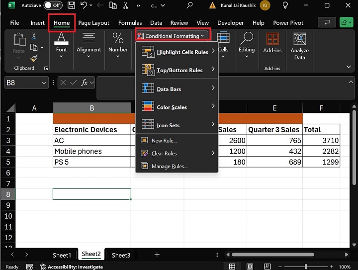
It can be difficult for beginners to find the Conditional Formatting button in Microsoft Excel. To find it, switch to the Home tab and select the Conditional Formatting button under the Styles group.
You can utilize the various built-in options, such as "Highlight Cell rules," "Top/Bottom Rules", "Data Bars", "Color Scales", and "Icon Sets" presented inside the Conditional Formatting button.
Use of Conditional Formatting in Excel
You may also set the New rule that contains Conditional Formatting Formula, Clear Rules, and Manage rules under the Conditional Formatting button.
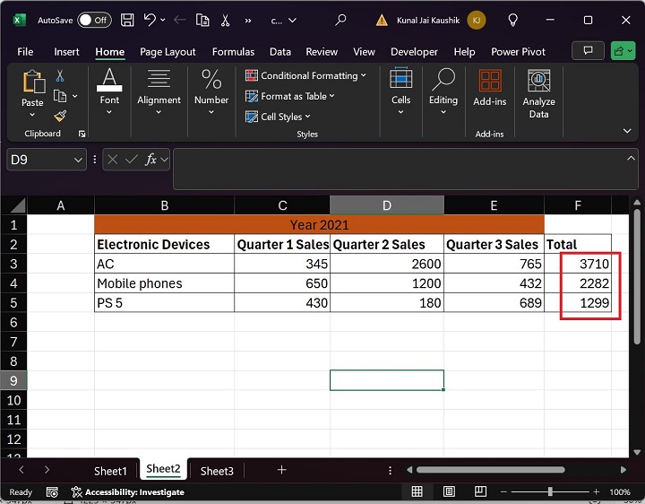
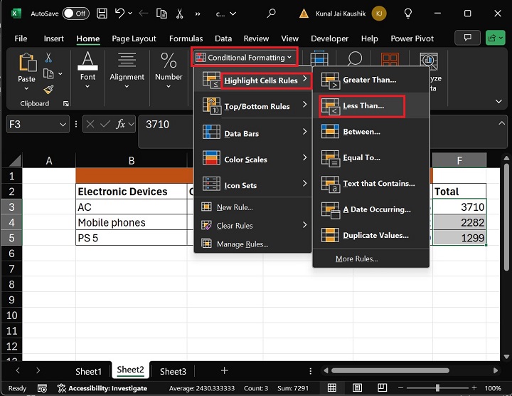
Lets say you wish to highlight cells with values greater than 2500 in the Total column. Select the cell range F2:F5, expand the "Conditional Formatting", select the "Highlight Cells Rules," and choose the "Less Than" option from the drop-down menu.
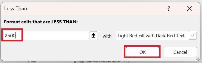
In the Less Than dialog box, specify 2500 in the "Format cells that are Less THAN:" section, select the "Light Red Fill with Dark Red Text" color, and click the OK button.
Therefore, the cells whose values are less than 2500 will be highlighted in a selected color.

Remove Conditional Formatting in Excel
- Open an active worksheet from where you intend to remove the conditional formatting.
- You can select the "Conditional Formatting" option, expand the "Clear Rules" from the drop-down menu, and choose any of the options, either "Clear Rules from Selected Cells" or "Clear Rules from Entire Sheet."
- The first option will be chosen if rules from the specified range of cells are being removed. If more than one rules/condition are defined earlier in the worksheet, then in that case, you can choose the "Cleat Rules from Entire Sheet".
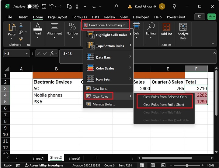
For instance, to remove Conditional formatting in the F column, first select the cell range F3:F5. Then select "Clear Rules from Selected Cells" as shown below −

Therefore, the conditional formatting has been removed from the F column.