How to highlight/conditional formatting dates older than 30 days in Excel?

By using conditional formatting, the user can color, highlight, or format cells dynamically, that depends upon the values, formulas, or rules the user defines. This feature is useful for some data points, patterns, or trends in the Excel worksheets, this makes the data easier to interpret and analyze the data. Instead of manually scanning through cells or applying to format individually.

This feature allows the user to automate the process and apply formatting dynamically as the data changes. In this article, users will learn the process of determining the number of dates older than 30 days in Excel. The first example will allow the user to understand the process of using conditional formatting with the help of the user−defined formula. While the second example allows users to calculate the dates older than 30 days with the help of kutools.

Example 1: To highlight or conditional format the dates older than 30 days by using the user−defined formula in excel.

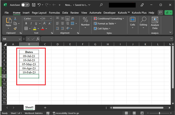
Step 1

First consider some sample date values, in dd-mmm-yyyy format. A snapshot for the same is provided below:

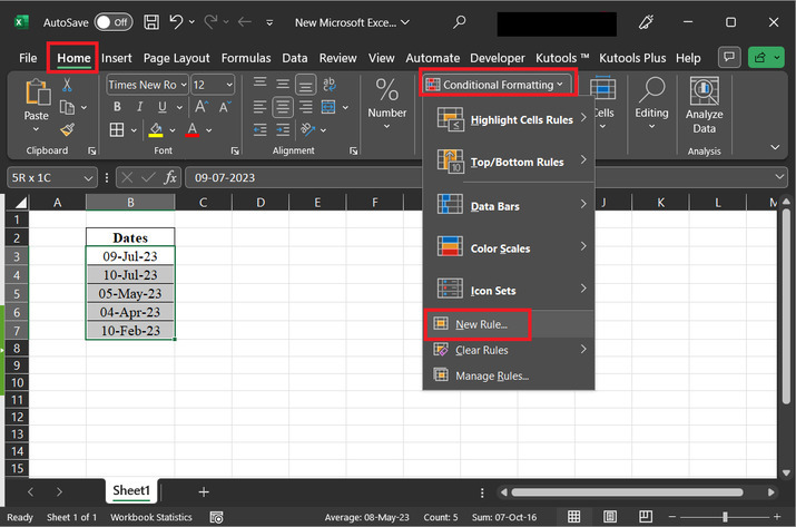
Step 2

First, select the data by clicking on all the available cells. After that go to the "Home" tab, and then select the "Conditional Formatting" option. Further, a new menu will appear. In the newly appeared dialog box, select the last third option "New Rule". A snapshot for reference is provided below:

Step 3

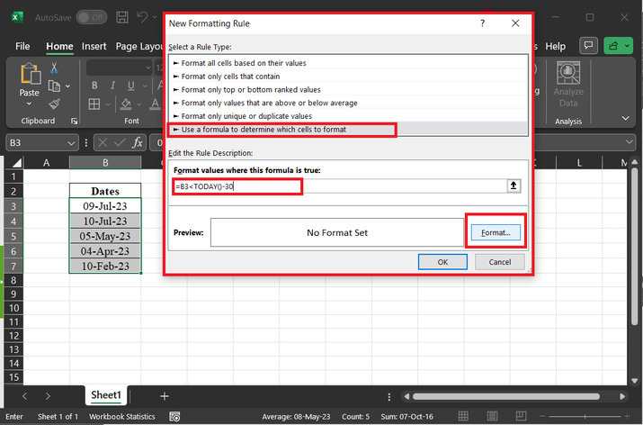
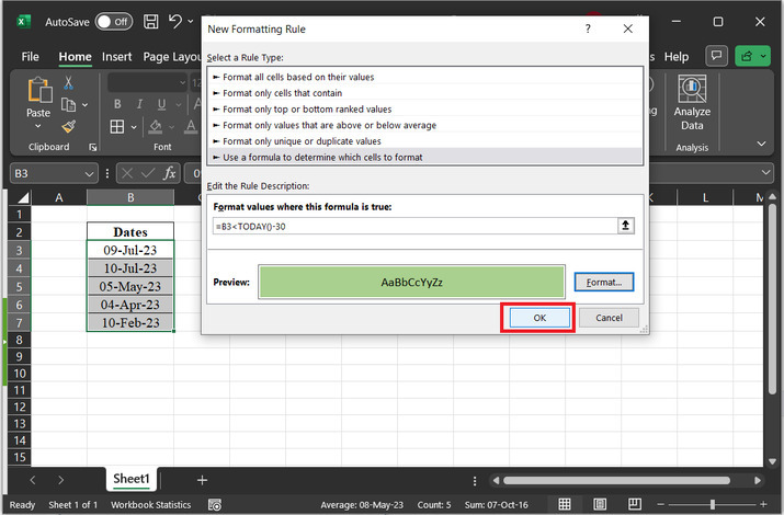
The other dialog box named "New Formatting Rule" will open. In the Select a Rule Type label, select the last option "Use a formula to determine which cells to format". After that move to the next input label, and type the formula "=B3<TODAY()−30". After that click on the "Format" button, provided at the side of the preview label.

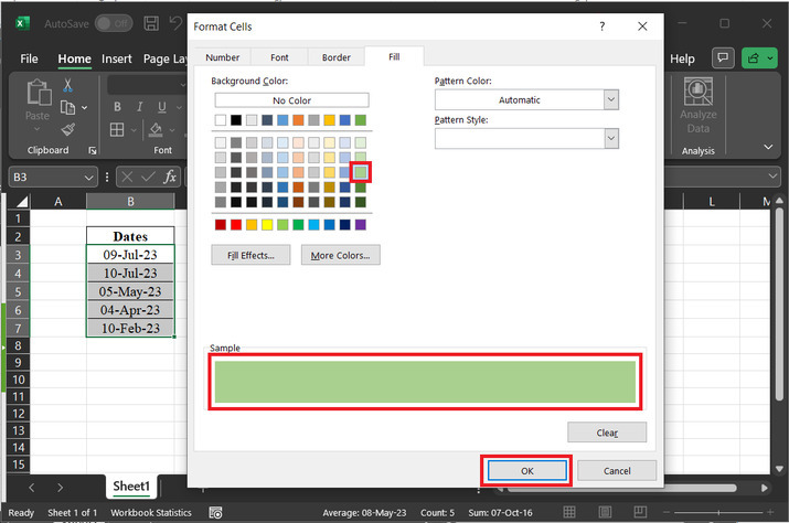
Step 4

The other dialog box named “Format Cells” would be displayed. After that click on the Fill tab, and in the background color option, the user can select the required green color. Finally, click on the “OK” button. snapshot for reference is provided below:

Step 5

The above−provided step will again display the “New Formatting Rule”. After that click on the “OK” button. A snapshot for same is provided below:

Step 6

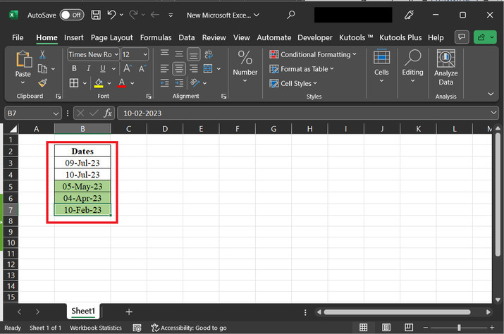
The above step will highlight all the dates that are older than 30 days. Snapshot for output is provided below:

Example 2: To highlight or conditional format the dates older than 30 days in Excel by using the kutools in Excel.

Step 1

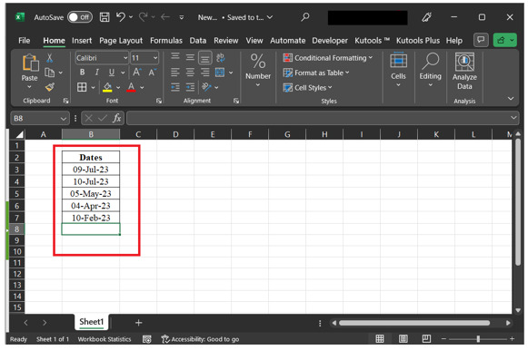
In this example, consider the dataset as highlighted below:

Step 2

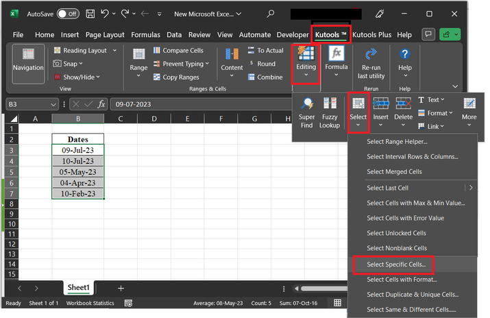
Go to the B column and select all the required cells. After that go to the “kutools” tab, and then choose the “Select” option. After that click on “Select Specific Cells”. A snapshot for reference is provided below:

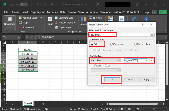
Step 3

The above step will open a “Select Specific Cells” dialog. In the opened dialog, go to the first input label, and select the required data range from B3 to B7. After that go to the “Selection type” label, and then click on the first radio button which is “cell”. Further, click on the specific type label, and set the drop-down to the “Less than” option. In the front input field set any date or select any date from the available “Data”. Further, click on the “OK” button. snapshot for user reference is depicted below:

Step 4

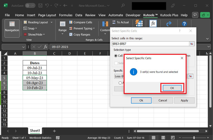
The above step will open a “Select Specific Cells” dialog cell. This dialog box, displays the count for the required results. After that click on the “OK” button. A snapshot for reference is provided below:

Conclusion

The above article contains a stepwise explanation for both the provided examples. The first example demonstrates the use of the user−defined formula, while the second example demonstrates the use of the kutools to obtain the older dates.