Conditional formatting rows or cells if two columns equal in Excel

When comparing and matching data in Microsoft Excel, you may do so in a variety of ways; however, the vast majority of these approaches focus on searching within a single column. When you compare and match data in Microsoft Excel, you can do so in a variety of ways. Instead of receiving the result in a separate column, which is something you may do if you want to highlight certain rows, conditional formatting enables you to highlight the rows that contain matching data. This can be done in place of getting the result in a separate column.

In this tutorial, you are going to learn how to use conditional formatting when two columns are equal.

Highlight Columns using Conditional Formatting

Using the conditional formatting feature of Excel, it is possible to compare two columns and highlight the Unique and Duplicate cells between them.

Let’s understand how it works, through an example.

Step 1

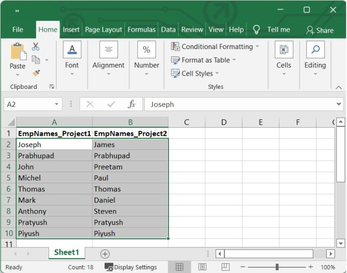
In our example, we have Employee names assigned for Project1 and Project2. There are some employees who are assigned for both the projects. We are going to compare both the columns and highlight those employee names who are assigned for both the projects.

See the following Excel sheet which contains the employee names for both the projects.

Step 2

Select the data in the columns to whom you want to compare. In our case, we are selecting the data from cell A2 to B10.

Step 3

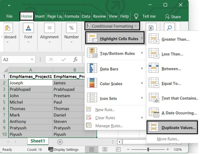
Now from the Ribbon, Go to Home Tab, then from the Styles group, select Conditional Formatting option. Then from the dropdown list, put cursor on Highlight Cell Rules, then go to Duplicate Values. (Home > Conditional Formatting > Highlight Cell Rules > Duplicate Values).

Step 4

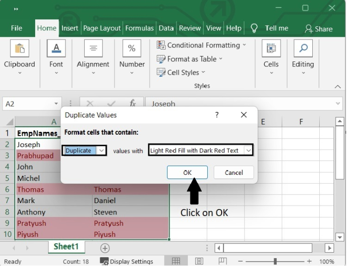
Now a popup window will appear. From the popup window, select Duplicate if you want to Highlight the duplicate data, otherwise select "Unique". In the place of "values with", select a color combination from the dropdown list appears as per your choice.

In our case, we are selecting Duplicate to highlight the duplicate data and values with as Light Red Fill with Dark Red Text. Then click OK.

Step 5

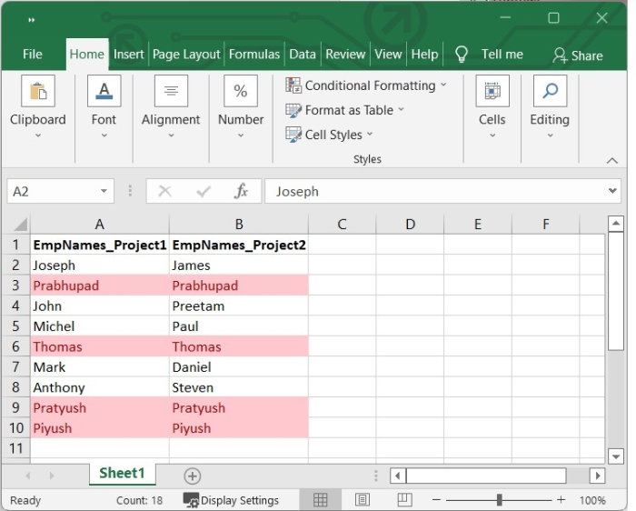
After clicking OK, we can see that the duplicate values have been highlighted with light red and dark red text.

Using Formula to format cells

You can use formula to highlight the duplicate data comparing both the columns. See the below given steps to use conditional formatting to the cell.

Step 1

We have the names of employees who are working on Project1 and Project2, listed here in our Excel sheet. Some of the employees are tasked with contributing to both of the projects.

Step 2

Select the data from the column you want to highlight.

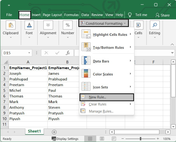
Now from the Ribbon, Go to Home tab, then from the Styles group, select Conditional Formatting option. Then from the dropdown list select New Rules option. See the below given image.

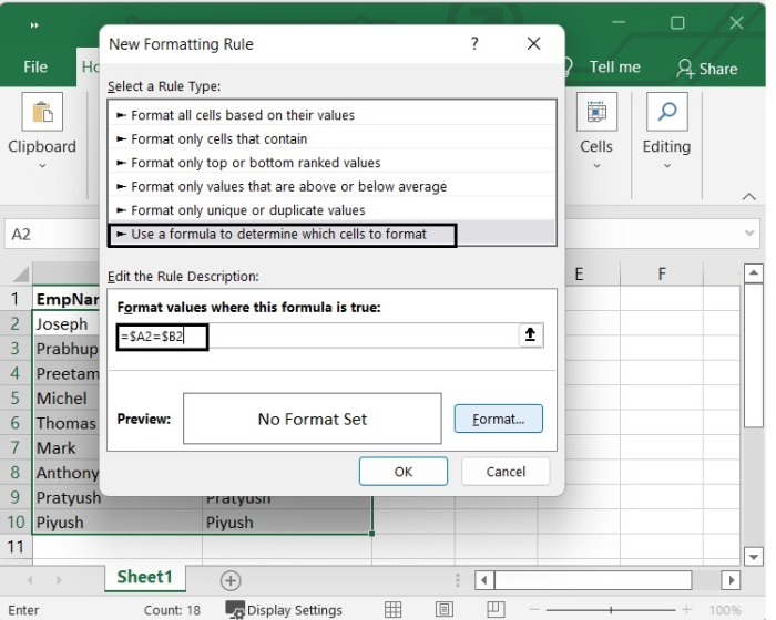
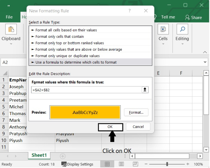
Step 3

In the New Formatting Rule dialogue, choose Use a formula to determine which cells to format from Select a Rule Type Section. Then, in the text box under Format values where this formula is true, type =$A2=$B2. We typed "=$A2=$B2" here because A2 is the first cell in the first list and B2 is the first cell in the second list we want to compare to.

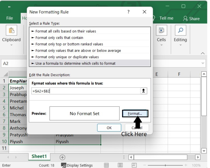
Step 4

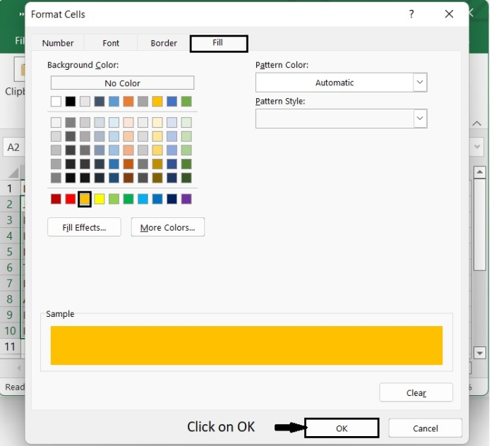
Click the Format button in the New Formatting Rule dialogue, then choose a background color in the Format Cells dialog's Fill tab. In our example, we have selected Yellow as background color with text color black. Then click OK.

Step 5

Now we can see that the duplicate data have been highlighted. See the image given below.

Conclusion

In this tutorial, you learnt how to use conditional formatting if two columns are equal. You can use any method as per your choice.